
Executive Summary
- Investors can use Credit Consensus Ratings to price risk in otherwise unrated names; but they can also use Credit Consensus aggregates to proxy risk for undisclosed Capital Relief Trades (CRT) portfolios.
- CRT portfolio credit risk can be proxied in a number of ways using Credit Consensus data – average default probabilities, proportions of names in very high yield categories (b and c).
- These metrics can be combined with market credit spreads to plot efficient frontiers and identify anomalies or scope for portfolio optimization; US Corporate bond spreads are closely correlated with aggregate average PDs and tail risk (% in b and c credit categories).
- Diversification benefits can be quantified by adjusting for correlations between aggregates. These correlations are more stable and potentially more meaningful than market-derived equivalents. Correlations between aggregates reduce measured portfolio risk in some cases by more than 20%.
- US Non-Life, Latin American Corporates and Belgian Corporates are the most diversifying aggregates. Regional and large country corporates are the least diversifying, followed by major US sectors. See Appendix for a return and risk chart for all (800+) aggregates.
- Risk estimates can also be adjusted by Point-in-Time stress scenarios. PIT adjustments approximately double the TTC default risk; the adjustment is larger for some higher risk portfolios.
- Risk estimates can also be adjusted by medium term credit transition rates. Long term transition effects increase risk by up to 5x, less for lower risk portfolios.
Risk sharing transactions (also known as Capital Relief Trades, Credit Risk Transfers, Significant Risk Transfers, Synthetic Risk Transfers, amongst other variations) are a rapidly growing asset class.
The sector has provided attractive risk-adjusted returns in the low-yield / low-default environment of the past decade; but global supply shocks and rising interest rates are expected to push corporate default rates higher.
For risk-sharing investors, emerging risks – and opportunities – highlight the need for timely and comprehensive credit data for accurate transaction pricing. This paper details how Credit Consensus Ratings and Aggregates provide a detailed map of the credit market risk-reward landscape, including possible anomalies.

1. Introduction
Europe has traditionally been the main source of risk sharing trades, but the US and Canada are increasingly important. Figure 1 shows the average geographic distribution of names from a small survey of (disclosed) CRT portfolios.
Figure 1.1 Average Geographic Distribution, Recent Disclosed Risk Sharing Portfolios
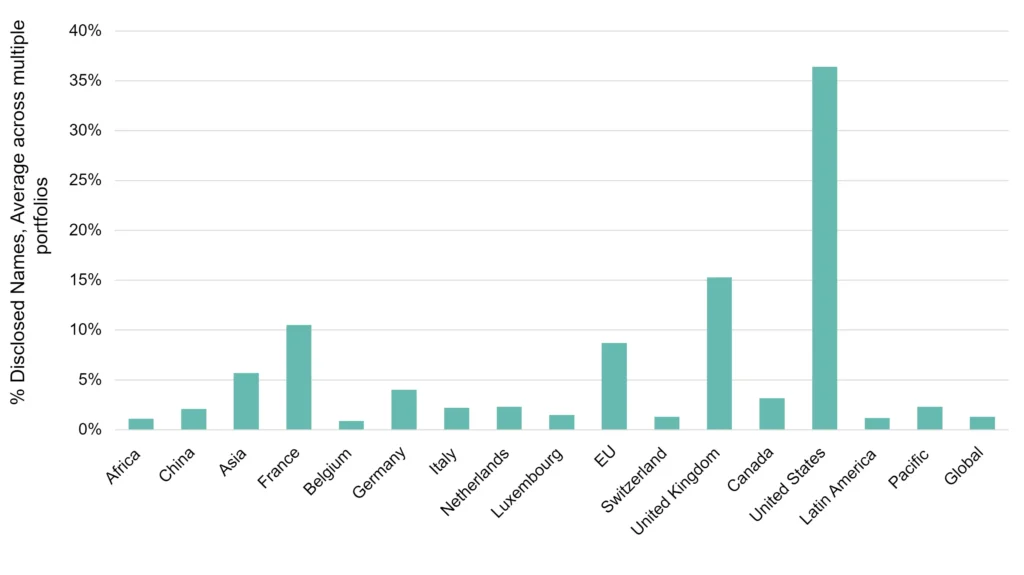
The geographic and sector diversity of CRT portfolios is a challenge for portfolio risk managers – a significant portion of the issuers involved are unrated, and in many cases the issuer names are not disclosed to investors. Credit Consensus data coverage includes many of the otherwise unrated corporates and financials that feature in risk-sharing transactions; it also shows detailed geographic and sector risk trends in the absence of detailed issuer information.
Risk sharing investors are a diverse group, with variable credit risk appetites and differing tolerances for transparency between disclosed and undisclosed lists of borrowers. Issuance of tranched investments (Senior, Mezzanine, First Loss) highlights the need for estimates of correlations between different credit categories and geography / industry combinations. Credit Consensus aggregates cover more than 1,200 such combinations and can be used to calculate correlations and PD volatilities at a granular country / sector level using recent or full cycle time series.
A subset of these aggregates are used in this note to compare several typical risk-sharing portfolios across a range of credit risk metrics. The outputs suggest that the Credit Consensus dataset may have significant value in the risk sharing segment.
2. Optimizing CRT Portfolios: Risk vs Reward Overview
Risk-sharing investment options are driven by banks who will aim to transfer assets that contribute heavily to their Risk Weighted Asset (RWA) calculations. If these are offered “blind”, the challenge for investors is to balance return against potential diversification benefit for their existing investments.
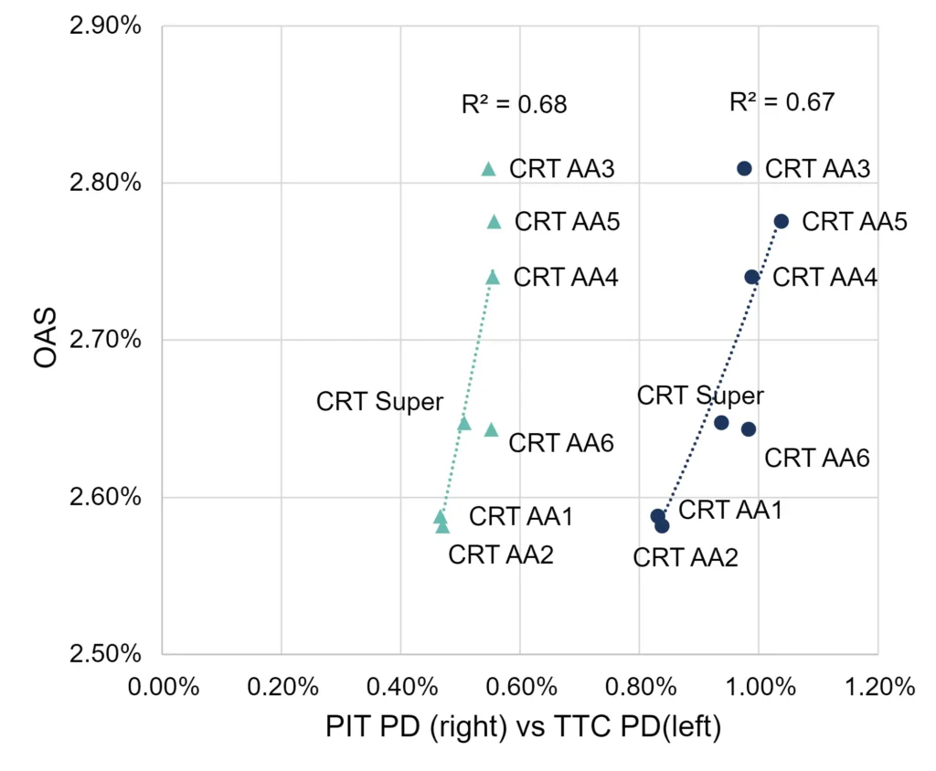
The classic approach to asset choice is to plot risk vs return for the asset universe. Figure 2.1 shows the relationship between Option Adjusted Spread[1] (OAS) as a proxy for return and Probability of Default (PD) as a proxy for risk, for a set of 30 geographic and sector aggregates used throughout this report.
Figure 2.1 Efficient Frontier 1: Spreads vs PD for 30 Geographic / Sector Aggregates
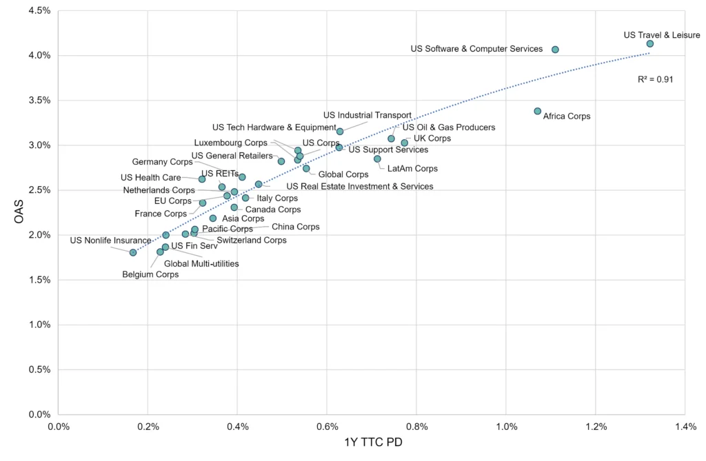
The correlation is positive and very high – so average credit risk for each aggregate is closely related to current OAS.
Similar correlations are likely vs CDS prices, secondary loan market rates, and most other traded credit assets, but these will be distorted by tranche structures. (At this stage, correlation between default risks is ignored – this is relaxed later in this report).
Figure 2.2 shows a similar chart with “Tail Risk” (% in b and c credit categories) as the risk measure.
Figure 2.2 Efficient Frontier 2: Spreads vs Tail Risk (% in b and c Credit Categories) – 30 Aggregates Used for Portfolio Examples
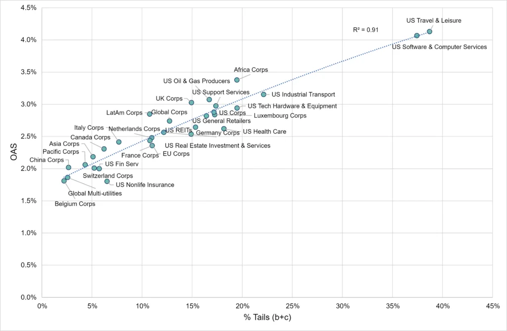
The correlation is again very high although the distribution of the aggregates in the plot is different. This suggests that any portfolio construction decisions need to use more than one risk metric.
The previous return vs risk charts ignore correlation between the various risk metrics for each aggregate. Credit Consensus data can be used to calculate correlations between PDs in terms of PD levels, PD changes, or the varying proportions of each aggregate in the tails (i.e. in the b and c credit categories).
Figure 2.3 plots the range of correlation estimates for each aggregate compared with the other 29 aggregates in the sample. Correlations use unweighted monthly data from 2016.
Figure 2.3 Most and Least Diversifying – 30 Aggregates Used for Portfolio Examples
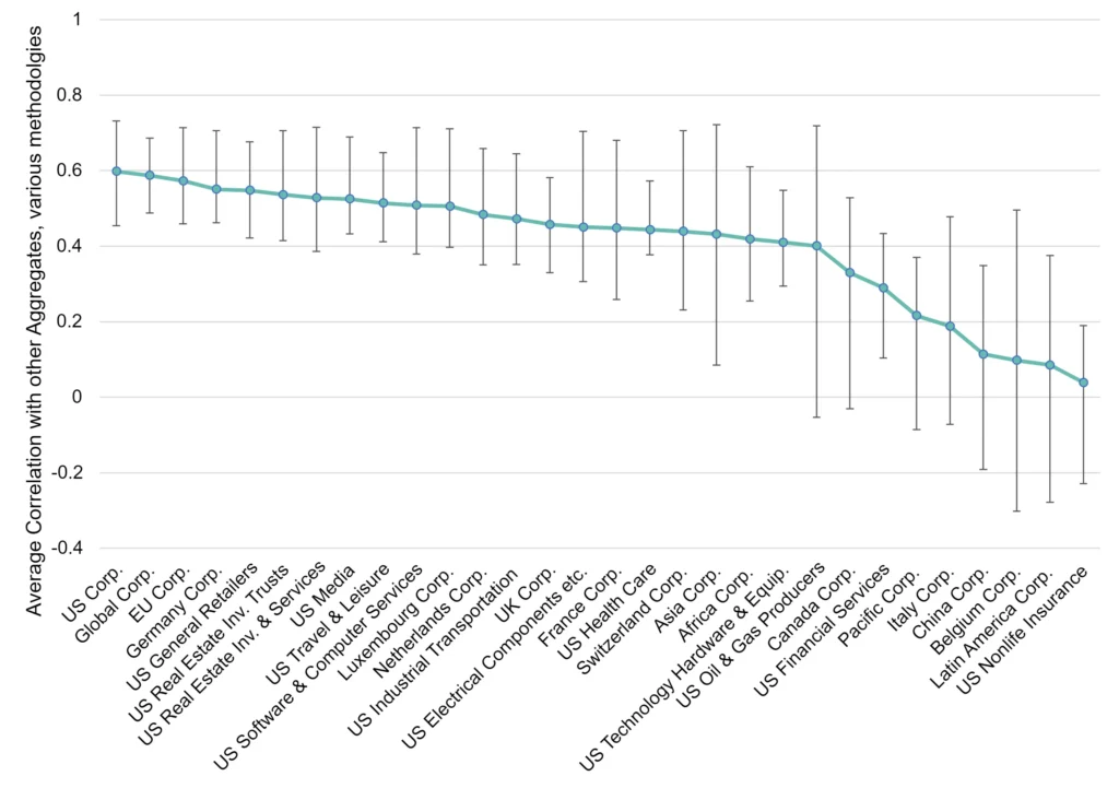
The error bars show the range of estimates using different measures of correlation – PD levels, PD Changes, and the proportion of aggregate constituents in the b and c credit categories.
US Non-Life, Latin American Corporates and Belgian Corporates are the most diversifying, although some of the error bars for these are wide. Regional and large country corporates are the least diversifying, followed by major US sectors.
Alternative sources of correlation estimates are patchy – CDS indices cover a limited range of names and many of them are illiquid; bond indices are more widely available but restricted to traded bond assets subject to the short-term swings in market sentiment and credit / liquidity risk premiums. Credit Consensus data provides a set of regular and consistent times series including risk estimates for legal entities that are not publicly traded. They are also stable over short periods, while showing trends and turning points over longer time periods.
Figure 2.4 shows rolling 12-month correlation between changes in US and European credit risk in the Healthcare sector, comparing Credit Consensus data aggregates with bond market-based proxies.
Figure 2.4 Rolling 12-month Correlation, US vs Europe Healthcare, Consensus vs Bond Indices
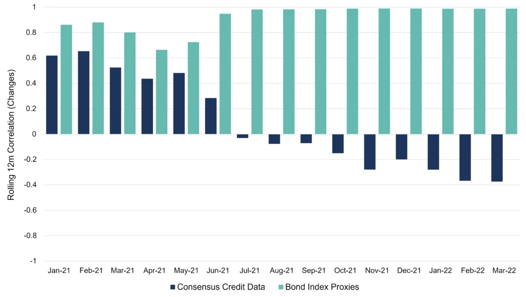
Credit Consensus data shows a much wider range in correlation estimates, dropping from 0.6 at the start of the period to -0.4 at the end. Over the same period, bond market proxies never dipped below 0.6 and were usually close to 1.
[1] The Option Adjusted Spread (OAS) is derived from recent (May 2022) OAS calculated by ICE-BAML and reported on the St. Louis Fed FRED website. The credit % distribution of the aggregate constituents across 7 categories (aaa, aa, a, bbb, bb, b and c) are used as weights to derive a weighted average OAS for each aggregate.
3. Portfolio Structures and the Typical CRT Portfolio
The sample portfolios used in this report have been selected to show how risk and return changes as the granularity of the exposures increases. This shows the value of mapping single names to aggregates, even with limited information (e.g. the country of risk is known but the industry / sector is not.)
Figure 3.1 shows allocations for each sample portfolio, with summary risk and return statistics.
Figure 3.1 Sample Portfolio Allocations and Summary Statistics
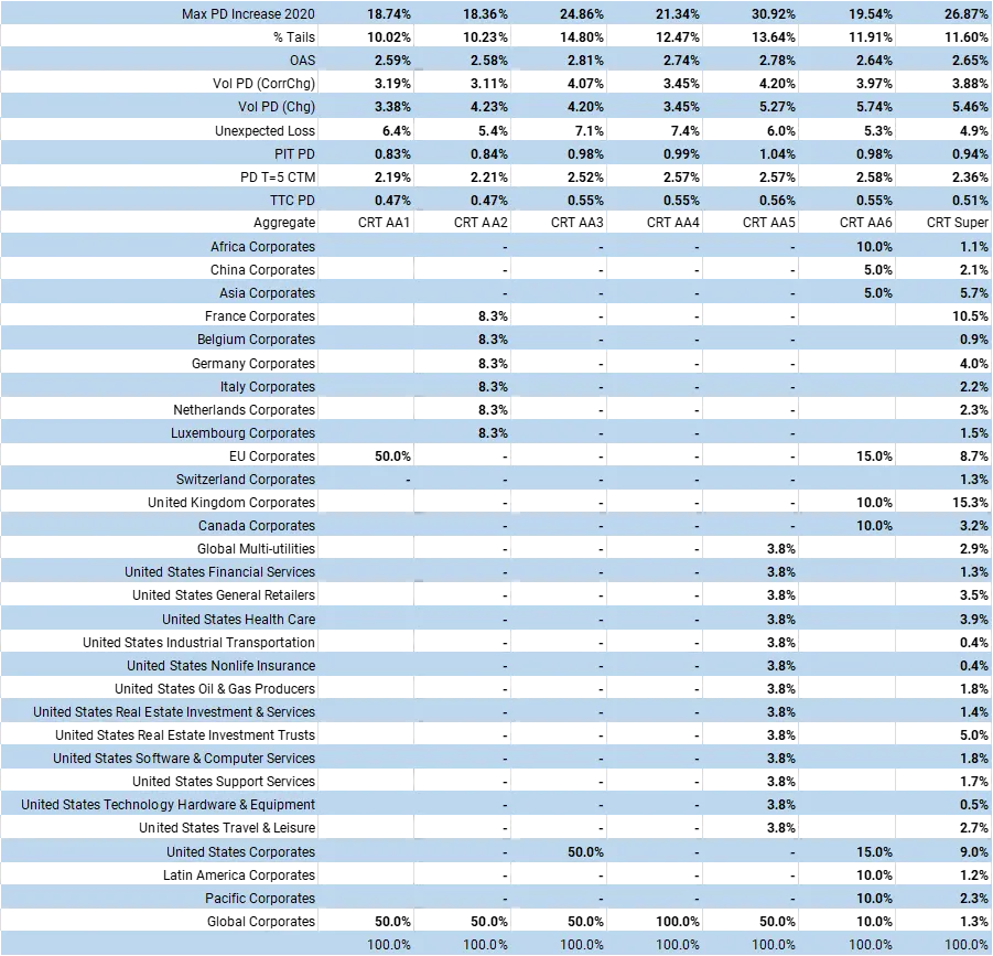
CRT Asset Allocation 1 (AA1) is a low-risk mix of 50 / 50 EU and Global Corporates, and AA2 splits the EU exposure by country. AA3 is a 50 / 50 mix of US and Global Corporates, while AA4 is 100% allocated to Global Corporates. AA5 again allocates 50% to the US, but splits this by sector. AA6 is a diverse geographic mix allocated by region. The final portfolio, “CRT Super”, is an approximate average of a number of disclosed portfolios – a more sector-detailed version of Figure 1.
Selection risk may be significant for any of these portfolios: aggregates cannot fully represent investor exposures in a particular sector or geography. The key issue is differences in credit behaviour between individual holdings and the typical aggregate constituent.
If, for example, investor exposures are all high yield in a specific sub-sector, their transition and PD change characteristics may be very different. This issue can be partly tackled by:
- Introducing “Selection” volatility and adjusting for the number of exposures (the higher the better)
- Adjusting for the % overlap between holdings and constituents (reducing the impact of maverick holdings)
- Modifying selection volatility to reflect the behaviour of the actual exposures
Selection risk is not included in these estimates but example calculations are shown in the Appendix.
Figure 3.2 graphs two of the sample portfolio on a radar chart, with each summary risk metric plotted on a different axis.
Figure 3.2 Radar Graph of Summary Risk Statistics for 2 Portfolios
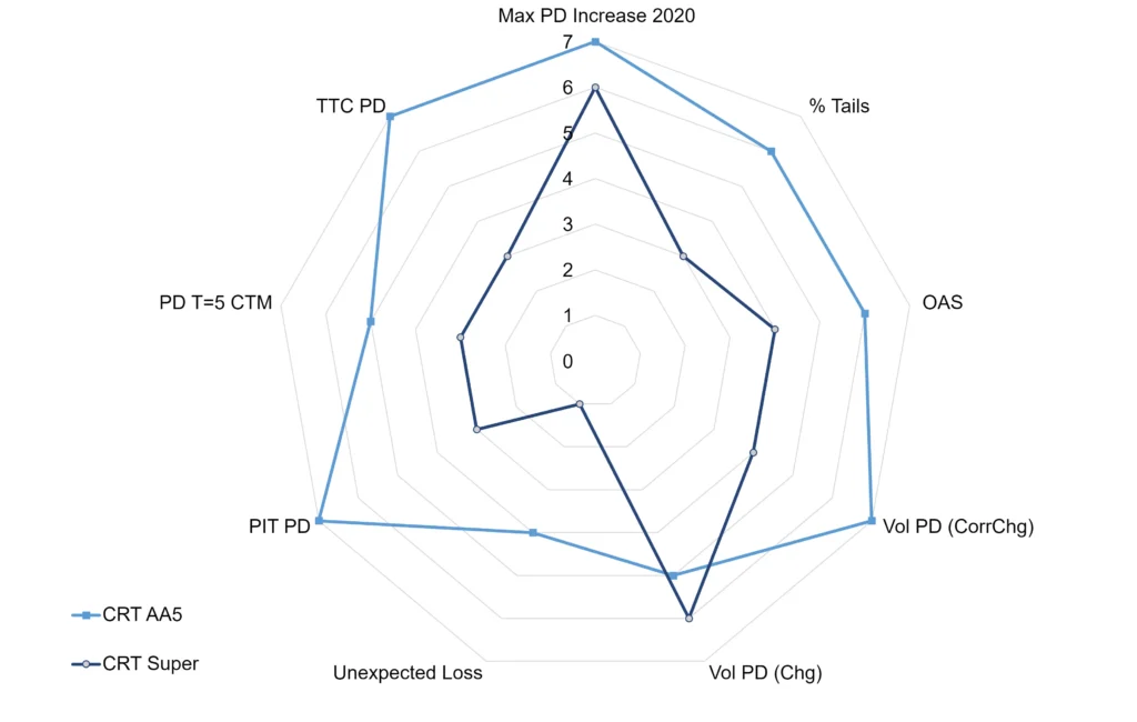
This shows that – compared with the CRT Super Portfolio, the AA5 is significantly higher risk on all of these metrics except for the Volatility without the Correlation adjustment. Multiple portfolios can be compared in this way.
Glossary of summary statistics reported for each portfolio in Figures 3.1 and 3.2
| TTC PD | Exposure weighted 1-year through-the-cycle ex ante probability of default. |
| PIT PD | Exposure weighted Point-in-Time ex ante probability of default |
| Vol PD (Chg) | Exposure weighted average of annualized standard deviation of TTC PD monthly changes |
| OAS | Credit category exposure weighted USD Option Adjusted Spread |
| PD T=5 CTM | TTC PD after 5th iteration of 1-year transition matrix |
| Unexpected Loss (UL) | Weighted average of [TTC PD * (1- TTC PD)]^0.5 (ie St.Dev. of Bernoulli distribution) |
| Vol PD (Corr Chg) | Exposure weighted average of annualized standard deviation of TTC PD monthly changes adjusted by monthly correlations between aggregates |
| % Tails | Proportion of portfolio in b and c credit categories |
| Max PD Increase 2020 | Change in PD in 2020 if portfolio held current exposures |
Case Study: Should Credit Portfolios Be Proxied by Country or by Sector?
The table below shows the summary risk statistics for two portfolios of US Corporate entities. The first maps all single names to the US Corporate aggregate; the second approximates the portfolio with 13 equally-weighted US Sector aggregates.
| Risk Metric | US Corporate = 100% | US = 13 Sectors |
| Max PD Increase 2020 | 28.4% | 40.5% |
| % Tails | 17.1% | 14.8% |
| OAS | 2.88% | 2.81% |
| Vol PD (CorrChg) | 4.95% | 5.26% |
| Vol PD (Chg) | 4.95% | 7.08% |
| Unexpected Loss | 7.33% | 4.96% |
| PIT PD | 0.96% | 1.09% |
| PD T=5 CTM | 2.47% | 2.56% |
| TTC PD | 0.54% | 0.56% |
The 100% US Corporate portfolio has a higher % in the tails and higher implied OAS; but on all other metrics it is lower risk.
The PD metrics are very close. PD volatility metrics are also similar but only after adjusting for correlations between sectors. The 2020 stress period has a much larger impact at the sector level.
This suggests that country exposures should be split into geographically specific sectors where possible to effectively capture risk extremes.
Figures 3.3 and 3.4 shows the relationship between OAS, PD, Tail Risks and Unexpected Loss for these 7 portfolios.
Figure 3.3 Spreads, Default Risks and Tail Risks for 7 portfolios
Figure 3.4 Spreads, Default Risks and Unexpected Loss for 7 portfolios
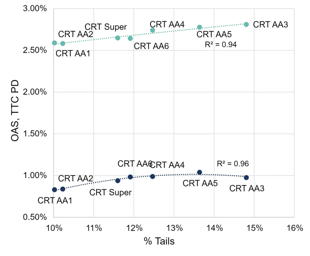
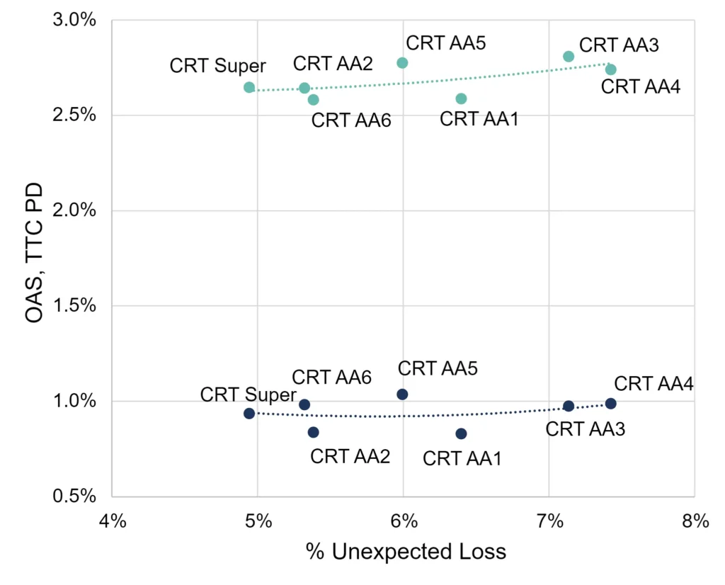
The % of aggregate constituents in the tails (b and c) are highly correlated with (1) the average PD and (2) the estimated spread.
The vertical difference between these two lines is roughly proportional to the combined Credit and Liquidity risk premium, adjusted by recovery rates.
It is worth noting that the Super portfolio is close to the middle of the sample based on % in the tails, but Unexpected Loss adjusted by Correlation makes the Super portfolio lowest risk. This suggests that using PD alone (and deriving Unexpected Loss (UL) from it) may understate the portfolio risk compared with other metrics.
4. Impact of Correlation
Figure 4.1 plots the relationship between the volatility of monthly PD changes over the period 2016-2021 for each of the 7 portfolios. The green bars show the weighted average volatility of the portfolio PD after adjustment for the effect of correlations between changes in aggregate PDs.
Figure 4.1 Relationship Between Volatility of Monthly PD Changes 2016-2021
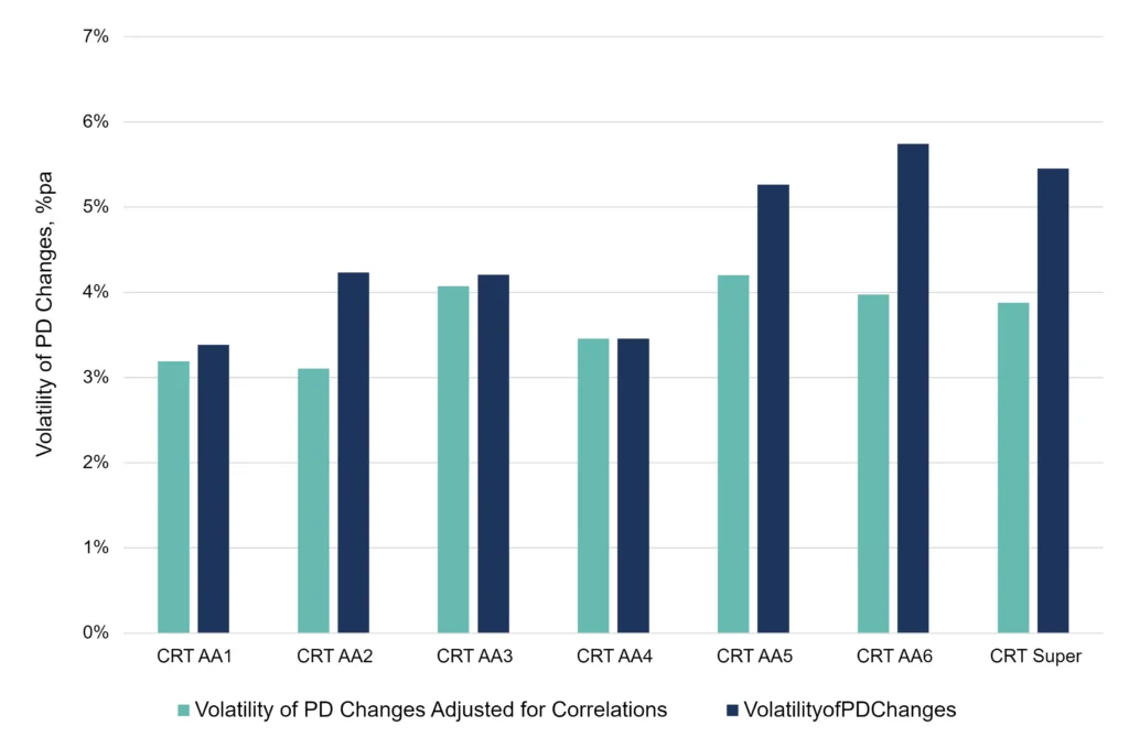
Apart from AA4, all portfolios show some reduction in PD volatility – marginal for AA3, but significant for AA5, AA6 and the “Super” portfolio.
[AA4 shows no correlation effect since it is represented by 100% exposure to Global Corporates.]
There are clear benefits to diversity and consensus aggregates can be used to quantify these.
Apart from AA4, all portfolios show some reduction in PD volatility – marginal for AA3, but significant for AA5, AA6 and the Super portfolio [AA4 shows no correlation effect, since it is represented by 100% exposure to Global Corporates.]
There are clear benefits to diversity and consensus aggregates can be used to quantify these.
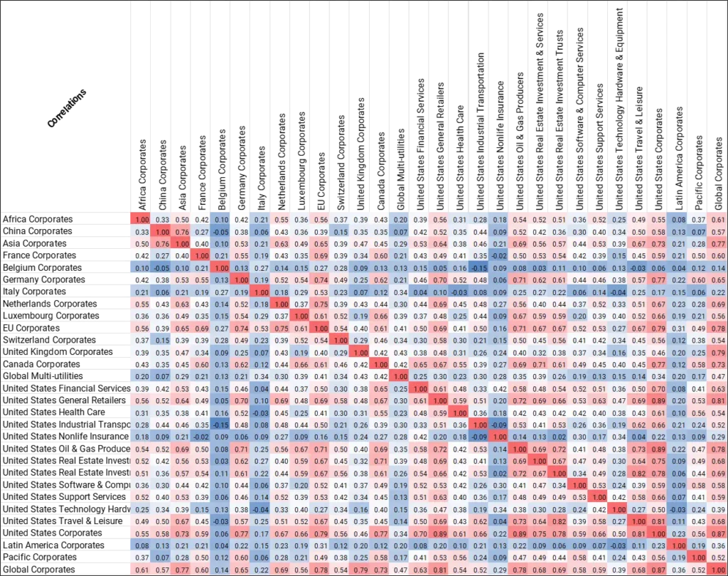
Figure 4.2 shows the correlations between PD changes for the 30 aggregates used in this report. Correlations can also be calculated using Levels, % in Tails, or asymmetric changes (i.e. just the PD increases). These usually give similar but not identical results, and for specific aggregates they may be very different.
Figure 4.2 Correlation between PD Changes
Extension to Tranche Correlations
Correlations between tranches can be estimated from the aggregates correlation matrix and the credit distributions of those aggregates.
If tranches are defined as Senior (aaa/aa/a), Senior Mezzanine (bbb), Junior Mezzanine (bb/b) and First Default (c), then a universe of aggregates can be used to proxy the correlations between tranches for a given underlying portfolio.
This first approximation can be refined by using the full universe of Credit Consensus aggregates to give more granularity, and by experimentation with the impact of defining the tranche boundaries – for example across 7 credit categories instead of three or four. See Appendix 8.1 for a description of the full universe of 800+ Credit Consensus aggregates.
For example, a number of emerging market aggregates (African Sovereigns, Turkish Banks) as well as sectors badly hit by COVID (US Travel & Leisure) have 10% – 20% of their constituents in the c category; while EU Sovereigns, North American Health Care and many developed market financials (including some Pension Fund aggregates) have very high proportions in the aa category.

5. Impact of Point-in-Time Adjustments
In banks and non-banks, Point-in-Time (PIT) credit risk models have been developed to address the need for impairment calculations under IFRS9 / CECL. These estimates complement the main Credit Consensus dataset, with stress test metrics showing how default risk changes in a downturn. These can be used to further differentiate and accurately price risk sharing portfolios.
Figure 5.1 shows the impact of PIT adjustments, specifically based on the period of credit stress at the start of the 2020 pandemic. These adjustments vary by industry and have been cascaded to the relevant sectors for each portfolio.
Figure 5.1 Impact of PIT Stress Scenario Adjustments on Through-The-Cycle (TTC) Risk Estimates
For a given level of OAS, each portfolio is shifted to the right as the PD is scaled up under the stress scenario. The correlations between OAS and PD remain almost unchanged for both metrics. However, risk for the higher return portfolios more than doubles while risk for the lower return shows a smaller increase. The greater impact of the PIT PDs for higher return portfolios is intuitive since their exposures bring higher tail risk.
6. Impact of Transition Adjustments
The impact of rising defaults can be measured using credit transition matrices – using Credit Consensus data these can be updated monthly, supporting decisions between long term and short-term holding strategies for specific groups of loans.
Figure 6.1 shows the impact of applying typical multi-year transitions to the 1-year PDs.
Figure 6.1 Impact of 5-year CTM Adjustments on PD Estimates
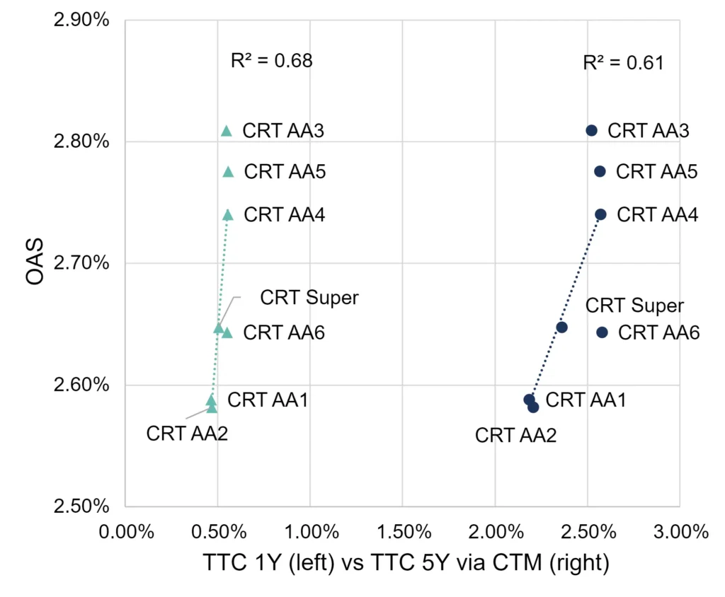
As before, for a given level of OAS, each portfolio is shifted to the right as the PD is scaled up; in this case the increase is the result of repeated transformations using a 7×7 credit transition matrix.
The correlations between OAS and PD are similar but lower in the 5-year case. The AA6 portfolio shows the proportionately highest increase in risk, while the highest return (AA3) and (especially) the lowest (AA2) show lower proportionate increases. This is due to the transition matrix effect, which pulls risky entities from both ends of the credit distribution into the center. However, the most risky portfolios increase by a factor of about 5x, while the least risky increase by about 4.5x.
To access the Foreword, Conclusion and Appendices of this whitepaper, please complete your details to download the full PDF report: