Whitepaper // No.7
November 2016
Transition Matrices

›Credit Benchmark crowd-sourced credit data is updated monthly and based on more than 250,000 obligors.
›Expert bank credit analyst views support a rich, diverse set of Ex Ante and Ex Post credit transition matrices.
›Through-the-Cycle data provides a valid base for transition matrix calibration and identifies path dependency.
›Real-world PD term structures provide risk premium adjustments for market implied Point-in-Time estimates.
›Term structure benchmarks optimize loan impairment calculations for IFRS9 and CECL accounting standards.
Download the PDF “Crowd-Sourced Credit Transition Matrices“
The latest CECL and IFRS9 accounting rules require banks and corporates to estimate potential losses over the entire life of a loan. Transition matrices can provide considerable insight into the likely pattern of losses over various time horizons.
Credit transition matrices (“CTMs”) are a key element in credit portfolio risk. Different sequences of upgrades, downgrades and defaults can lead to very different portfolio outcomes.
Credit rating agencies are the main current source of transition matrix data, typically publishing separate high-level matrices for corporates and financials in the main geographies. These matrices provide a summary of the rating activity of each agency.
This paper compares bank-sourced transition matrices with the traditional estimates published by the main credit rating agencies (“CRAs”). It shows that the crowd-sourced data is comparable with agency data, but it is also published more frequently, and provides some insight into the key question of path dependency in rating migrations.
It also uses the crowd-sourced transition matrices to estimate ‘Real World’ Probability of Default (“PD”) term structures, and shows how these compare with ‘Risk Neutral’ or Market-Implied term structure estimates. This has implications for Point-in-Time (”PIT”) and Through-the-Cycle (“TTC”) estimates.
| Credit Benchmark: Collective Intelligence for Global Finance | |
| Credit Benchmark (CB) has brought together a group of key global banks who anonymously and securely pool their internal credit risk estimates, to create consensus Probabilities of Default (“PD”) and senior unsecured Loss Given Default (“LGD”) metrics. The Credit Benchmark service offers monthly updated consensus PDs and LGDs on thousands of obligors at the individual legal entity level, extending from Sovereigns and banks to public and private corporates and funds. Credit Benchmark also offers data on tens of thousands of obligors for use at portfolio level. Quorate consensus PDs are simple, unweighted averages of at least three independent PD or LGD contributions for an identical legal entity over an equivalent estimation period. Participation in the service is open to any banks, which use the IRB method for calculating regulatory capital. Credit Benchmark warmly invites interested institutions to become contributors. |
A credit transition matrix (“CTM”) is a key element in credit portfolio risk 1 . Different sequences of upgrades, downgrades and defaults can lead to very different portfolio outcomes.
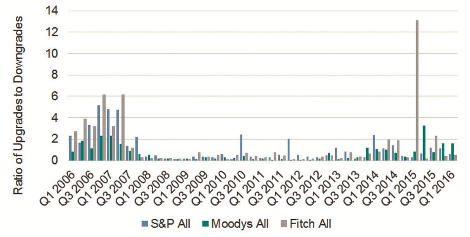
Credit rating agencies are the main current source of CTM data, typically publishing high-level CTMs as a summary of their annual rating activity, separately for corporates and financials, in the main geographies. Rating changes tend to be clustered in time 2 so in some years the reported CTMs may be based on sparse underlying data.
Crowd-sourced credit estimates 3 provide a robust complementary source of data. The underlying data consists of tens of thousands of forward looking credit risk estimates provided by large numbers of expert credit analysts in global IRB banks. These estimates benefit from the so-called “Wisdom of Crowds” 4 and are updated frequently. The very large underlying dataset also offers a new and unprecedented level of granularity.
Users of CRA or crowd-sourced data need to be aware of the distortions arising from smoothing and sampling variation. The observed transition matrices can be viewed as a record of ‘Ex Post’ transitions in a fixed set of obligors over a specific time period. There is an ‘Ex Ante’ equivalent, which is the theoretical pattern of transitions that would be expected for obligors of the same type. This can be calibrated to the behavior of Probabilities of Default (“PDs”). These matrices can then be used to estimate Cumulative Probability of Default (“CPD”) term structures, providing a benchmark for comparison with market implied term structure measures of default risk.
In this report, we use crowd-sourced data to estimate the broad dimensions of a number of CTMs. We also show PD volatility data at detailed levels of credit quality granularity; PD volatility can be used to simulate Ex Ante CTMs. We compare key statistics for crowd-sourced CTMs and rating agency CTMs. The crowd-sourced CTMs are then used to derive cumulative PD term structures, which can be compared with market-implied measures.
We also discuss the issue of path dependency and show how high frequency time series credit data can be used to assess serial correlation in PDs. This gives an indication of the impact of serial correlation on the structure of the CTM and the implications for term structure estimation.
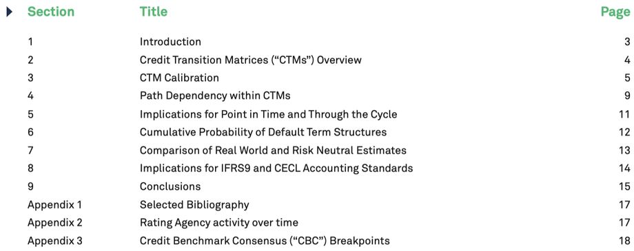
A Credit Transition Matrix (“CTM”) published by rating agencies shows the frequency (in %) of upgrades and downgrades from one credit category to another over a specified period (typically updated annually, with the cumulative changes also calculated for longer periods).
Exhibit 2.1 illustrates the process and shows the key components of a CTM. The histogram on the left shows a typical distribution of obligor credit quality. If these obligors are subject to a series of credit quality transitions over time, then the distribution will change – for example to the histogram shown on the right. In the center of the diagram are the key components of the credit transition matrix itself. The upper right triangle of the CTM (‘Down’) is the frequency of downgrades for each row, and the lower left triangle (‘Up’) is the frequency of upgrades for each row. The largest value in any row is nearly always the diagonal element (‘Stable’), which shows the percentage of obligors in each rating band whose credit rating does not change in the chosen period. The actual default frequency appears in the final column (D). The bottom row (‘Emerge’) shows the frequency with which obligors emerge from default.
Exhibit 2.1: Typical CTM and Credit Quality Distributions
For example, the number of AAA companies in the world has fallen dramatically in the past 20 years, and most of these have moved to AA+, then to AA, and so on. Multiple notch moves are possible following the Brexit vote, S&P downgraded the UK Government by two notches from AAA to AA.
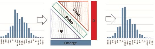
Exhibit 2.2 shows the S&P 30 year experience for Global Corporates, averaged to give the ‘typical’ single year experience.
Exhibit 2.2 S&P Long Run CTM
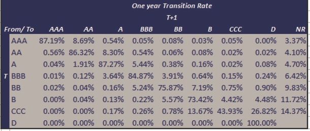
Exhibit 2.2 shows that the number of companies that started and ended each year rated as AAA by S&P is 87.19%. 5 In a typical year, 8.3% of the obligors rated as AA at time T (left hand) are downgraded to A at time T+1 (top row). This value is shown in row ‘AA’ and column ‘A’. CTMs often include a Default category (column ‘D’ at the far right), so the rows add up to 100%. The table also shows that in a typical year over this 30-year period, 4.48% of the obligors rated as B had defaulted by the end of the year. (Row ‘B’, Column ‘D’). This matrix includes a ‘Not Rated’ column, showing how often companies of different credit classes drop out of the rating process. Row ‘D’ is constructed to have zeros on all off-diagonal elements; so in this matrix ‘Default’ is an absorbing state. In practice, companies sometimes emerge from default (especially those with Chapter 11 status in the USA).
Throughout this paper, the individual entries in the CTM are referred to as cells and they are identified by the row, and the column, respecitvely. In the CTM above, cell (AAA,AA) = 8.69%. Cells which are not on the leading diagonal are on the 1st, 2nd, 3rd etc. diagonal.
Exhibit 3.1 provides a detailed comparison of the diagonal element values of the S&P data shown previously along with the crowd-sourced data for the 12 months to July. These elements show the proportion of obligors in a given credit category which remain in that category after one year. Although these percentages represent observed frequency, they are usually interpreted as probabilities.
Exhibit 3.1 Actual 1-year Probability of No Transition: Global Corporates, 12m to July 2016
This shows that both datasets demonstrate an increased likelihood of transition for lower quality credit categories. It also shows that, with the exception of the AAA category, the Credit Benchmark crowd-sourced CTMs show higher transition likelihoods across the credit spectrum.
Although the crowd-sourced and CRA data show differences, the crowd-sourced estimates are based on a very large, robust cross-sectional sample which should minimize noise. The CRA data is based on a robust combination of time series and cross sectional data, so it should also contain limited noise. However, the history potentially straddles very different credit regimes, and the CRA data will reflect the desire by CRAs and their clients to avoid volatility in credit ratings.
Exhibit 3.2 shows a comparison of the key elements of the S&P CTM from Exhibit 2.2, and the crowd-sourced equivalent, 1-year transition frequency, averaged across credit categories, for the 12 months to July 2016 6 .
Exhibit 3.2 Comparison of S&P and Crowd-sourced CTMs, 12 months to July 2016
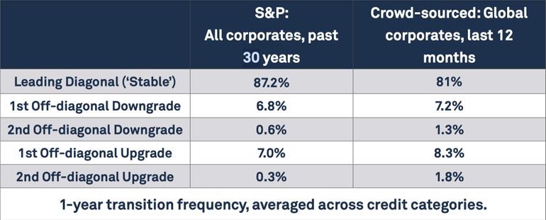
This shows that crowd-sourced data shows a tendency to more activity (up or down) and in particular a bias towards upward revisions over this period. It also shows that crowdsourced 2nd diagonal elements (two notch transitions) are higher than the S&P equivalent.
Exhibit 3.3 shows a comparison of the crowd-sourced CTMs for different geographies and different types of obligor, 1-year transition frequency, averaged across credit categories.
Exhibit 3.3 Comparisons of crowd-sourced CTMs by geography and type, 12 months to July 2016
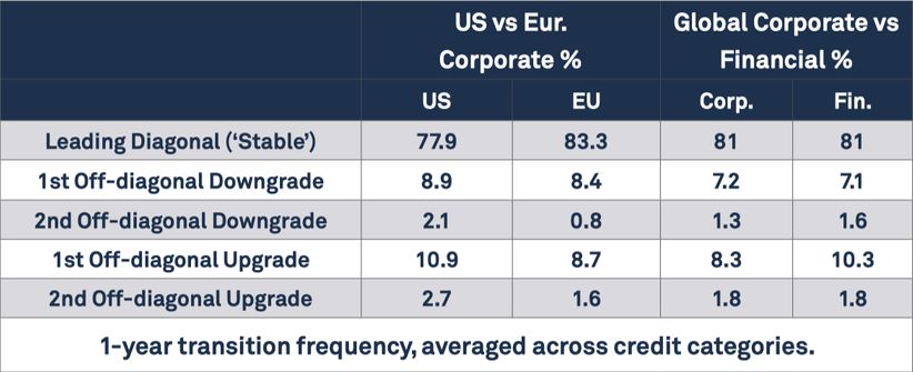
This shows that US Corporate obligors show transitions more often in all categories. It also shows that the frequency of upgrades is slightly higher than the frequency of downgrades for both Europe and US. It shows that Corporates and Financials have very similar transition propensities, except for the one notch upgrade diagonal.
Exhibit 3.4 shows the Ex Post 21 x 21 CTM for US Corporates.
Exhibit 3.4 Ex Post 21 x 21 CTM, US Corporates, 12 months to July 2016
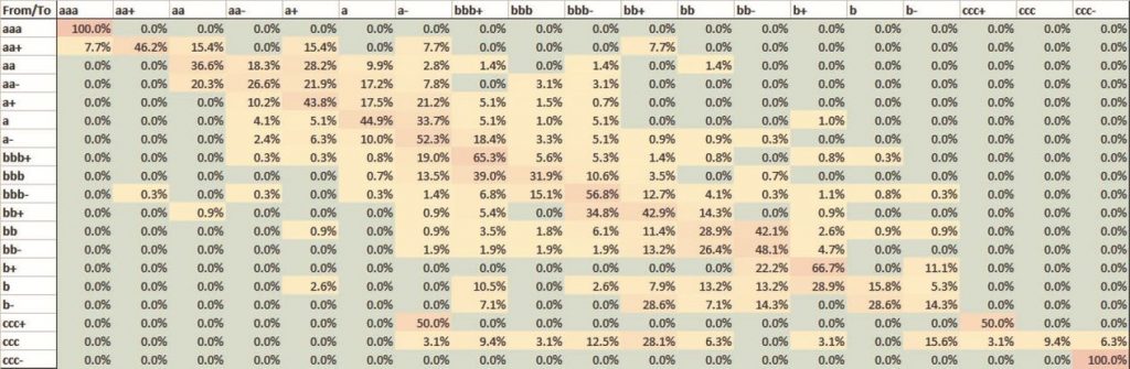
This shows that the crowd-sourced dataset now contains sufficient data to begin to populate a 21 x 21 Ex Post CTM. This CTM is still subject to significant noise, especially in the highest and lowest credit categories, where there are fewer obligors. However, this noise level is steadily dropping; and the PD volatility approach described in the next section offers additional scope to simulate and calibrate an Ex Ante CTM for benchmarking purposes. As the database continues to expand in terms of breadth, depth and history, it is expected that the number of credit categories can be expanded further.
Developers and users of transition matrices often smooth the data to ensure ‘monotonicity’. There are various approaches, but all produce the result that cells on a given row that are further from the leading diagonal show progressively lower values. Monotonicity is not guaranteed in raw data and deviations from monotonicity are regularly observed in crowdsourced data. This is mainly because of sampling variation, especially when the sample period is short. However, monotonicity can also be violated by major credit events, such as large jumps from investment grade into high yield, or even into default.
Users of CRA or crowd-sourced data need to be aware of the distortions arising from smoothing and sampling variation. The observed transition matrices can be viewed as a record of Ex Post transitions in a fixed set of obligors over a specific time period. There is an Ex Ante equivalent, which is the theoretical pattern of transitions that would be expected for obligors of the same type.
The key driver of any transition matrix is the volatility of the credit views. In CRA data this is determined by the changes in the opinions of the agencies. In crowd-sourced data, the proportionate volatility of the PDs 7 will determine the scale and frequency of transitions. The other driver is the frequency with which that volatility is relevant – i.e. the frequency with which PDs change or not. This has a significant impact on the leading, ‘Stable’ diagonal. In addition, the ‘jump to default’ process can arguably be viewed as an extreme form of PD volatility; but could also be viewed as a separate discrete event process.
Exhibit 3.5 shows the results of a simple CTM simulation model based on proportionate PD volatility.
Exhibit 3.5 CTM simulation results for different proportionate Monthly PD volatility levels
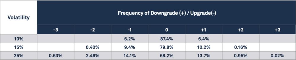
This shows that higher PD volatility results in more frequent and larger notch transitions. Proportionate PD volatility can be tracked every month across a range of obligor types, regions and sectors. This can be used for systematic monitoring of forthcoming changes in CTM behavior.
This table can be used in reverse to infer the PD volatility level that prevailed over the estimation period for a CTM. This involves a comparison of the key diagonals of the CTM with the rows in the above table, interpolating where necessary.
In particular, it is possible to use different PD volatility assumptions for different credit categories; this allows close replication of the higher transition frequencies observed in the lower credit quality obligors.
This simulation approach can be used to construct an Ex Ante CTM, which exhibits limited noise. This in turn provides a set of benchmarks for observed Ex Post CTMs, and gives risk practitioners a clearer view of the amount of smoothing required.
Exhibit 3.6 shows some estimated Proportionate PD volatilities for various obligor subsets.
Exhibit 3.6 Proportionate PD Volatility estimates, 6 month time series window
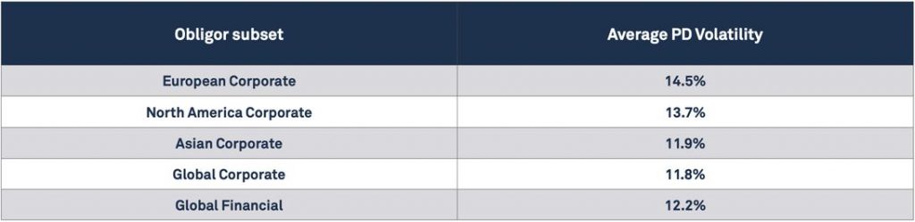
This suggests that the average PD Volatility is similar across the obligor subsets, but – for example – Global Corporates are closer to the first row of Exhibit 3.5 and European Corporates are closer to the second row. Note that these estimates are based on a 6-month volatility window, whereas the estimates in Exhibit 3.3 are based on 12-month transitions. This is the reason for European Corporates appearing at the top of this table, while European Corporates show fewer transitions in Exhibit 3.3.
Individual obligors show much greater variation in PD Volatility. As Exhibit 3.7 shows, this is mainly a function of credit category.
Exhibit 3.7 Proportionate PD Volatility (Monthly) estimates by Credit Category
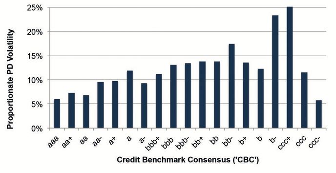
This shows that, as an approximation, each credit notch adds about 1 percentage point to the monthly PD Volatility. PD volatility is generally higher but also much more unstable in the non-investment grade categories. This partly reflects the smaller sample of obligors, but also reflects genuine uncertainty about the credit outlook for low quality obligors, leading to larger and more frequent revisions in PD estimates. This helps to explain the higher propensity to transition observed in lower quality obligors.
Path dependency is a major issue in applying CTMs. Path dependency implies that the relevant CTM for each obligor is conditional on the previous credit behavior of that obligor. If an obligor has been downgraded in one period, then that obligor becomes more likely to downgrade in the next period.
If credit behavior is path dependent, then two portfolios with the same initial distribution of obligors across credit categories may evolve in very different ways, depending on the previous upgrade/downgrade behavior of the individual obligors in each portfolio.
Exhibit 4.1 shows the CBC-7 8 distribution of obligors by credit category after (rather unrealistically) 20 years of upgrades, downgrades and defaults 9 . (This is derived by multiplying the transition matrix by itself, and then multiplying the result by the original transition matrix a further 19 times).
Exhibit 4.1 20-year Derived Distribution (Global Corporates i.e. CTM used in Exhibit 3.2)
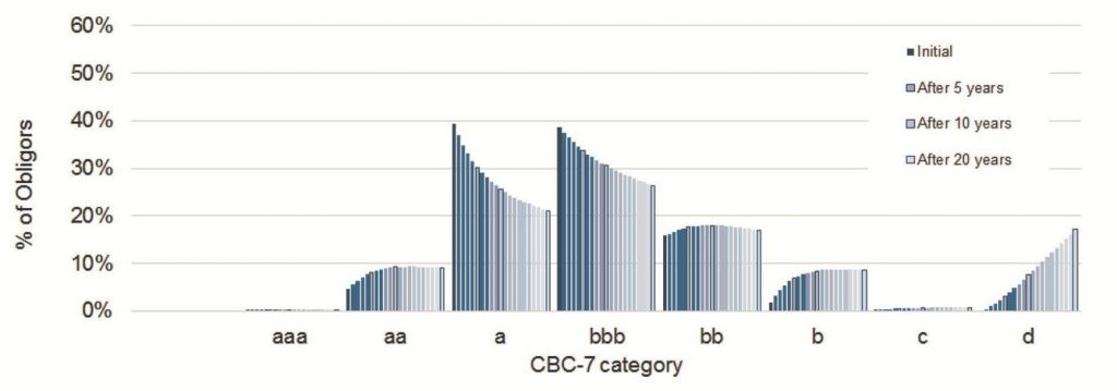
The initial distribution is based on the current obligor set in the Credit Benchmark dataset; this is consistent with the generally bell-shaped curve that is observed in credit rating distributions (a Normal distribution is usually a good approximation).
The final distribution (after 20 years) is significantly different, with fewer obligors in a and bbb categories, and more in aa and b categories. The bb and c categories show an initial increase, but then show a slight decline.
This type of chart is useful for summarizing the behavior of an individual transition matrix. In the example in Exhibit 4.1, the current matrix does not preserve the current obligor distribution. This may be because the current distribution is unusual, or (more likely) because the current distribution is typical but is generally preserved by a combination of:
Exhibit 4.2 shows the incidence of path dependency in the monthly CB dataset.
Exhibit 4.2 Runs in PD Changes, Credit Benchmark and Simulated Data
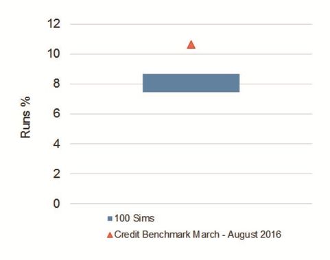
This shows that, for a subset of the quorate corporate data, the proportion of non-zero PD changes where the sign is the same in two subsequent months is 10.6%.
In 100 simulations of a similar, sparse dataset where each PD change is independent by construction, the proportion is in the range 7.4% 8.7%. This suggests that the actual PDs show ‘Runs’, which is a weak form of path dependency.
Subset of Obligors where n>=7
The impact of path dependency on obligor distributions will depend on the nature of the additional transition matrices that come into force as a result of an upgrade or downgrade. Typically we would expect the number of obligors accumulating in the higher or lower quality or default categories will be higher than would be achieved by simply powering up the observed, unconditional CTM. This is because for every unconditional CTM, there is a family of nested, conditional CTMs that apply to obligors that have just experienced an upgrade or downgrade. A more general approach to this is described in Bluhm and Overbeck (see Appendix 1). They relax the assumption of time homogeneity but retain the Markov assumption. In effect, the transition probabilities change over time. 10
The Credit Benchmark dataset is based on ‘Through-the-Cycle / Hybrid’ estimates; so the PD for each obligor reflects the average risk throughout a full credit cycle, with adjustments for changes in circumstances which affect the outlook for specific sectors or individual obligors.
The Through-the-Cycle (‘TTC’) estimate is the 1-year equivalent of the full cycle, cumulative PD estimate 11 . This means that CTMs based on the one-year estimates are generally (surprisingly) suitable for providing multi-year cumulative PD estimates and term structures.
Point-in-Time (‘PIT’) estimates are conditional on the current state of the credit cycle. Since they are typically calibrated with direct reference to market prices (CDS and bond yields), they will contain a market risk premium, of which liquidity is usually the dominant element.
The risk premium provides a bridge between TTC and PIT. There is evidence from Sovereign CDS markets 12 that this risk premium varies over time and is a function of credit quality, so it can be tracked and systematically used to convert between these two measures. It also has a term dimension, which in the case of PIT can be observed in market prices and yield curves, and in the case of TTC it can be derived from the CTM. The next section discusses this in more detail.
This section assumes that the crowd-sourced CTMs are unconditional (i.e. universally applicable, since they are based on TTC data). It should be noted that conditional CTMs might provide more accurate term structures that take the changing credit regime into account. Exhibit 6.1 shows the 5-year cumulative PD term structure derived from the unconditional CTM using the Global Corporate CTM for S&P and crowdsourced data. Due to the scale mismatch, only the investment grade PDs are plotted.
Exhibit 6.1.1 S&P
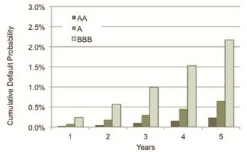
Exhibit 6.1.2 Crowd-sourced
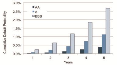
This shows that, using the crowd-sourced data, an obligor who is classed as bbb at the beginning of the period has a probability of more than 2.5% of defaulting after 5 years. The S&P data shows a value of just over 2.1%. S&P also publish multiple year CTMs and these may give different results, but this specific result shows that the S&P data reflects a range of credit regimes over the past 30 years, whereas the crowd-sourced data reflects the changes in TTC views over the past 12 months. N.B. Obligors who default after 5 years may have remained in the bbb category throughout the period up to the default, or they may have upgraded and downgraded in the process of reaching a default state.
These probabilities are calculated using a full transition matrix. An alternative is the survival approach, which ignores the process of upgrades and downgrades – in effect, a diagonal CTM. Exhibit 6.2 compares these two approaches for aaa, bb, and c credit categories.
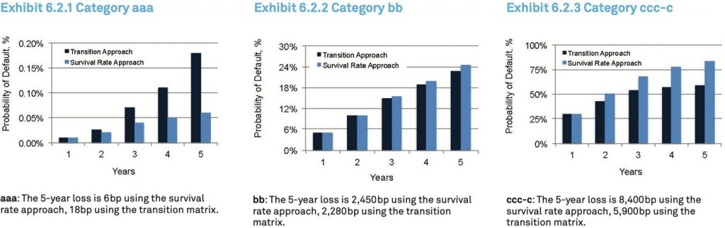
This shows that the two approaches give very different estimates of default probabilities at different time horizons. It also shows that there is a crossover point somewhere between bbb and bb. For credits of bbb and better, the survival approach understates the cumulative probability of default; for credits of bb or worse, the survival approach overstates the cumulative probability of default. This is because the cumulative PD for the aaa credit class curves up; the c class curves down.
The difference between ‘Real World’ and ‘Risk Neutral’ probabilities can be significant, with implications for the different Probability of Default use cases. For example, for the purposes of accounting standards covering loan impairment (see section 8, below) it is important to use real world PDs.
Risk neutral PDs consist of real world PDs plus an allowance for risk premiums, especially liquidity risk premium. This reflects the market maker’s need to be compensated for providing liquidity, and the need for the investor to be compensated for holding an illiquid asset. The other main source of risk premiums is counterparty risk – this is especially prevalent in CDS prices. Risk neutral PDs are primarily a pricing concept, and are subject to a broader range of influences than those of a real world PD. Baxter & Rennie give a good example of this in their ‘Parable of the Bookmaker’:

The liquidity premium is increasingly important for insurance companies. Solvency II rules require explicit recognition of asset liquidity, so any source of robust estimates of the liquidity risk premium will allow insurance companies to more accurately reserve capital. Real World PDs are key to estimating the proportion of an observed credit spread that can be attributed to liquidity, and the extent of reserving required.
Exhibit 7.1 Comparison of Real World and Risk Neutral (Market Implied) PDs.
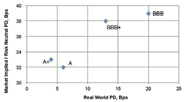
Exhibit 7.1 shows Real World and Market Implied PDs for four credit classes, based on a sample of US Corporate Bonds. The difference can be substantial, depending on the prevailing risk premium. When market implied default probabilities are used, it is important to take the current risk premium into account to avoid overstating potential losses. (Where losses are being hedged using traded instruments, (e.g. CDS) then the risk premium will be part of the cost of the position and will be included in the net profit or loss.)
These standards require recognition of loan impairment over multiple time periods. The CECL 13 rules (applicable to US entities) require a full assessment of the likely impairment of a loan over its lifetime, whereas the IFRS9 14 rules (applicable to non-US entities) only require multiple time horizon estimates when the credit standing of a loan has deteriorated significantly. Global banks will generally have to report under both standards depending on the domicile of the lending subsidiary.
15 , a lending entity should:›apply the CECL model for financial assets measured at amortized cost, such as loans, debt securities, and any receivables that represent the contractual right to receive cash;
›assess the collectability of contractual cash flows, using information about past events, current conditions and reasonable and supportable forecasts;
›consider all contractual cash flows over the life of the related financial assets (i.e. the loan)
›estimate expected credit losses reflecting the risk of loss, even when that risk is remote
›use methods to estimate expected credit losses which may include:
Exhibits 6.2.1. – 6.2.3 and Exhibit 7.1 show that the assumptions made about transition matrices and the choice of PD are critical to loan impairment estimates. For the aaa category, the transition matrix approach gives a 5-year loss estimate which is 3 times higher than the survival rate approach. For the c category, the transition matrix approach results in a 5-year loss estimate that is 30% lower than the survival rate approach. (Other CTMs will have less dramatic but nevertheless significant impacts on impairment estimates.) The market implied PDs in Exhibit 7.1 are 1.5 – 6 times the magnitude of the Real World probabilities.
For CECL and IFRS9 accounting, the choice of CTM and default probabilities is crucial and may have a significant impact on the final reserving required. This paper has demonstrated some of the key issues in choosing credit transition matrices:
The Credit Benchmark dataset is a large and frequent source of credit risk updates. The dataset tracks all such changes across the mapped universe (which exceeds 250,000 names) for a variety of time periods (one month to one year).
Through-the-Cycle data is well suited to the calibration of transition matrices with multiple time horizons and provides fresh insights into the path dependency issue.
The resulting transition matrices can be used to estimate cumulative PD curves and provide benchmarks for Point-in-Time risk estimates derived from market prices. These can then be used to estimate monthly risk premiums for different obligor types, credit classes and time periods.
These benchmarks have applications for compliance with IFRS9 and CECL accounting standards, and the choice of CTM and PDs may have significant financial implications. In particular, crowd-sourced CTMs provide:
Crowd-sourced CTMs provide a flexible and frequently updated set of building blocks for a variety of regulatory and accounting use cases across the banking and insurance industries.
Financial Calculus: An Introduction to Derivative Pricing: Baxter M & Rennie A (1996)
Markov Model for the Term Structure of Credit Risk Spreads: Jarrow, RA, Lando, A and Turnbull SM (1997)
From Default Probabilities to Credit Spreads: Denzler S Dacorogna M Muller U, McNeil A (2005)
Calibration of PD Term Structures To Be Markov or Not to Be: Bluhm C Overbeck L (2006)
Credit Rating Dynamics and Markov Mixture Models: Frydman H Schuermann T (2007)
Credit Migration Risk Modeling: Andersson, A. Vanini P (2010)
On the Risk Neutralization of Transition Matrix: Zhou, R (2013)
Current Expected Credit Loss: A New Impairment Model Is Born: C. Henkel (Moody’s Analytics / GARP) (2016)
Download the article “Crowd-Sourced Credit Transition Matrices” on PDF.
We aggregate the views of thousands of institutional credit analysts to create new, unique consensus data and analytics. Our clients use the unique entity- and aggregate-level data and analytics to understand and manage their risks effectively. The data helps clients focus their attention on where and when it matters most, whether in their risk management, investment process, or regulatory compliance. Learn more.
Barbora Makova
Jacob Hibbert
Aleem Ilyas
David Carruthers
1 See Appendix 1 for a brief selection of the large literature on this topic.
2 See Appendix 2.
3 The Credit Benchmark (“CB”) dataset covers thousands of obligors at the individual legal entity and portfolio levels. Data is collected monthly from key global banks who anonymously and securely pool their internal credit risk estimates. From these, CB create consensus Probabilities of Default (“PD”) and senior unsecured Loss Given Default (“LGD”) metrics.
4 The ‘Wisdom of Crowds’ was initially observed by Francis Galton and is the basis for the value in crowdsourced datasets. It is the popular version of the Diversity Prediction Theorem which can be stated as: “The squared error of the collective prediction equals the average squared error minus the predictive diversity” – implying that if the diversity in a group is large, the error of the crowd is small.
5 In practice, some companies may go through multiple downgrades (or upgrades) in the course of a year. The CTM in Exhibit 2.2 represents a specific time horizon (one year, in this case). More generally, the transition process can represented by a continuous time-homogenous generator matrix which generates the discrete time CTM(t) = exp(Gt) where CTM(t) is the credit transition matrix at time t and G is the associated generator matrix. Generator matrices are useful but computation may be complex – see, for example, Moler, C. and van Loan, C. “Nineteen Dubious Ways to Compute the Exponential of a Matrix, Twenty-Five Years Later.” SIAM Rev. 45, 3-49, 2003
6 These rows do not sum to 100%, due to defaults; these matrices have also been rebased to conform to one set of default rates for each credit category.
7 Proportionate PD volatility is defined as the rolling standard deviation of the obligor PD estimates over a set time window, divided by the average PD for that obligor over the same period. The choice of rolling window will have some bearing on the estimate.
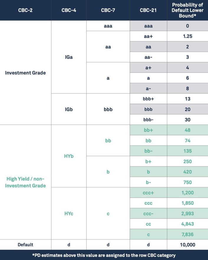
8 CBC-7 refers to the aaa, aa, a,bbb,bb,b,c categorization. See Appendix 3 for the full table.
9 This distribution ignores company births. In practice, large numbers of companies are incorporated each year (the ONS in the UK report typical annual birth rates in the range 13 – 14%, and typical overall death rates (across all credit categories) of 3.5% – 6%).
10 For the purposes of this paper, we note that path dependency is likely to be an issue, but it is not incorporated into the derived metrics in sections 6 and 7 below. Current Credit Benchmark and Technical Advisory Group research is focused on the implications of path dependency for CTMs and Cumulative PD terms structures, with results forthcoming. This is aimed at formulating and calibrating CTMs which are consistent with (1) observed default frequencies (2) observed credit category distribution of obligors through time.
11 Typically this means that if the credit cycle length is assumed to be 5 years, and the 5-year PD is given by PD(5), then the one-year PD or PD(1) = (1-(1-PD(5))^(1/5)). In other words, the PD(1) is derived from the 5th root of the 5-year survival probability.
12 See Credit Benchmark White Paper No.4, available to download from www.creditbenchmark.com
13 CECL = Current Expected Credit Loss.
14 IFRS = International Financial Reporting Standards.| Crowd-sourced Credit Transition Matrices
15 FASB = Financial Accounting Standards Board. These guidelines were published in
Credit Benchmark is an entirely new source of data in credit risk. We pool PD and LGD estimates from IRB banks, allowing them to unlock the value of internal ratings efforts and view their own estimates in the context of a robust and incentive-aligned industry consensus. The resultant data supports banks’ credit risk management activities at portfolio and individual entity level, as well as informing model validation and calibration. The Credit Benchmark model offers full coverage of the entities that matter to banks, extending beyond Sovereigns, banks and corporates into funds, Emerging markets and SMEs.
We have prepared this document solely for informational purposes. You should not definitely rely upon it or use it to form the basis for any decision, contract, commitment or action whatsoever, with respect to any proposed transaction or otherwise. You and your directors, officers, employees, agents and affiliates must hold this document and any oral information provided in connection with this document in strict confidence and may not communicate, reproduce, distribute or disclose it to any other person, or refer to it publicly, in whole or in part at any time except with our prior consent. If you are not the recipient of this document, please delete and destroy all copies immediately.
Neither we nor our affiliates, or our or their respective officers, employees or agents, make any representation or warranty, express or implied, in relation to the accuracy or completeness of the information contained in this document or any oral information provided in connection herewith, or any data it generates and accept no responsibility, obligation or liability (whether direct or indirect, in contract, tort or otherwise) in relation to any of such information. We and our affiliates and our and their respective officers, employees and agents expressly disclaim any and all liability which may be based on this document and any errors therein or omissions therefrom. Neither we nor any of our affiliates, or our or their respective officers, employees or agents, make any representation or warranty, express or implied, that any transaction has been or may be effected on the terms or in the manner stated in this document, or as to the achievement or reasonableness of future projections, management targets, estimates, prospects or returns, if any. Any views or terms contained herein are preliminary only, and are based on financial, economic, market and other conditions prevailing as of the date of this document and are therefore subject to change. We undertake no obligation to update any of the information contained in this document.
Credit Benchmark does not solicit any action based upon this report, which is not to be construed as an invitation to buy or sell any security or financial instrument. This report is not intended to provide personal investment advice and it does not take into account the investment objectives, financial situation and the particular needs of a particular person who may read this report.