
Table of Contents
1. Introduction
2. Credit Risk Portfolio Framework: Overview
3. Extension to Multiple Indices
4. Transaction Analysis
5. Portfolio Optimization
6. Conclusion
7. Credit Index Portfolio Risk – Worked Example
1. Introduction
Global debt is mainly held in credit portfolios by banks, insurance companies, investors, private companies, as well as some governments. These investors make extensive use of credit agency ratings and market-driven risk models.
Other segments are faced with less visibility: large corporates need credit portfolio management to handle often unrated supplier or customer default risk. And the growing risk-sharing business – where one financial institution agrees to underwrite the credit risk of another – is also portfolio based. This segment includes undisclosed portfolios where one counterpart may agree pricing without detailed knowledge of the individual constituents.
Credit portfolio management models have a long history backed by extensive academic literature, but in practice they are only as good as the credit risk data available to them.
The portfolio management objective seems simple: maximize returns subject to an acceptable level of risk. Estimates of gross return (before defaults and recoveries) are often possible with a high degree of accuracy. But the net return – after adjusting for defaults and recoveries – has a high estimation error, although robust data can reduce that uncertainty.
Historic default data is notoriously patchy, but forward-looking consensus data can cover the gaps. This paper reviews a data-driven framework for portfolio risk analysis and discusses practical applications of consensus credit risk estimates.
The appendix gives details of calculation formulas. An Excel workbook is also available with example calculations – these can be tailored to individual client asset universes.
2. Credit Risk Portfolio Framework: Overview
NB: The framework discussed here is not a substitute for detailed analysis of individual company balance sheets, cash flows, and legal status. It aims to provide a context for portfolio decisions where underlying names are not disclosed or difficult to analyze due to incomplete data. The Appendix discusses metrics that adjust portfolio credit risk according to the number of single loans in each portfolio.
Bank loan books are diversified across multiple borrowers, but the risk reduction benefit is limited when credit portfolios are concentrated (e.g., in one country or industry). This can be tackled with industry / country concentration limits, although these can be subjective.
But if borrowers are grouped by geography and industry, portfolio risk can be measured via estimated default correlations between obligor groups. Group choice matters: risk estimates derived from industry-level metrics may not match a detailed sector-based view.
The ideal framework allows a risk manager to assess how risk estimates change with different industry or geographic mappings. A useful portfolio-level metric is PD[1] volatility, a proxy for credit migration risk – i.e. upgrades, downgrades and defaults. This metric can be calculated by combining portfolio profiles with consensus credit data.
The ideal framework allows a risk manager to assess how risk estimates change with different industry or geographic mappings. A useful portfolio-level metric is PD volatility, a proxy for credit migration risk – i.e., upgrades, downgrades, and defaults. This metric can be calculated by combining portfolio profiles with consensus credit data.
Example: The Global Travel & Leisure (T&L) sector suffered multiple downgrades during Covid, while the Global Software (SW) sector benefited from online shopping and working from home.
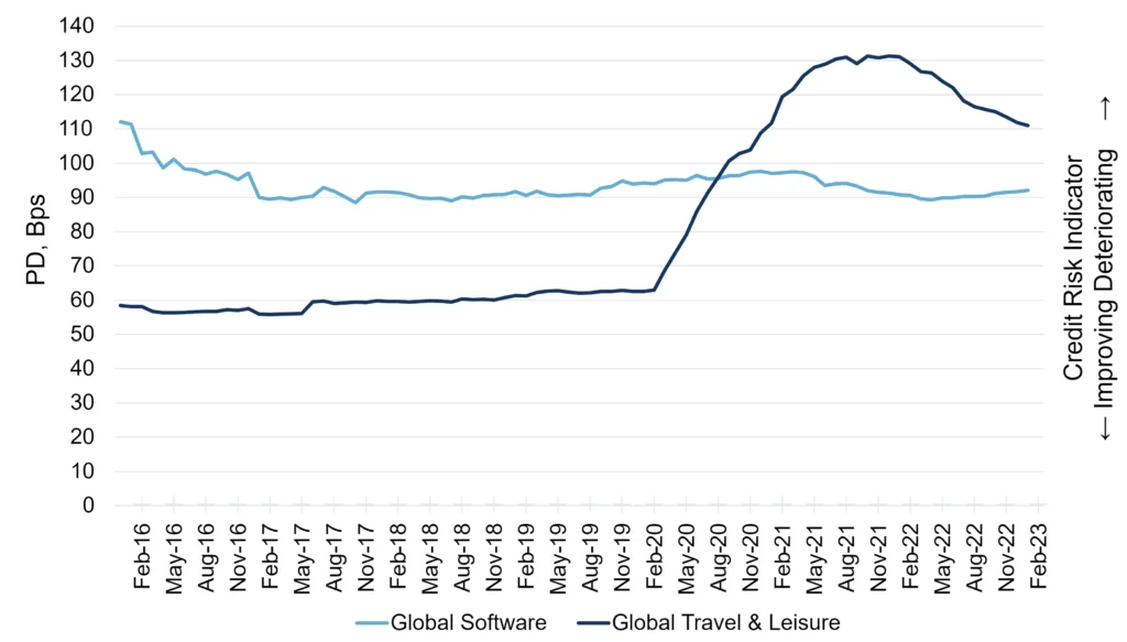
The chart shows that – from the onset of the pandemic – T&L average default risk rose from 63 bps to 131 bps, while SW stayed in the range 71-80bps. For a credit portfolio with 50% in each sector, the average PD would have moved within the narrower range of 67 to 104. Similar results can be seen in the monthly standard deviations of the PD changes, which are 1.2% and 3.3% for the sectors and 2.1% for the portfolio, with monthly correlation of 0.45[2].
This approach can be extended to multiple regions, countries, industries and sectors. Standard deviation / correlation metrics also have the advantage that they can be used for estimating the marginal contribution to risk of each additional loan.
3. Extension to Multiple Indices
The image below shows correlations between monthly PD % changes for global sectors, plus the average PD level and PD volatility of each index.
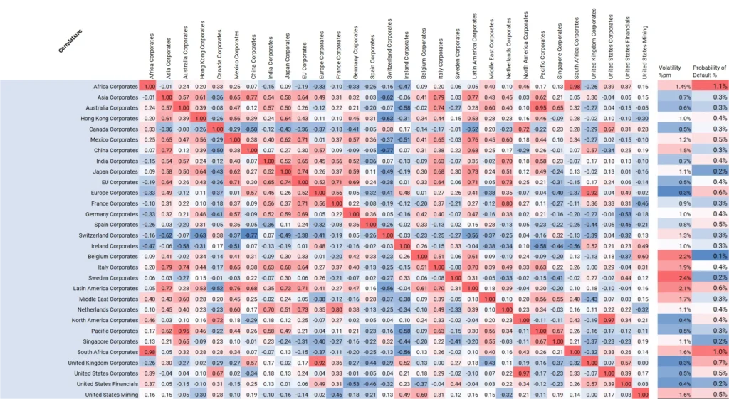
This matrix is based on the past 12 months. Such a truncated period can reveal some very divergent short-term trends. Italy, for example, shows a high correlation with Asia (+0.79), higher than its correlation with Germany (+0.40). Switzerland is negatively correlated with many other indices, with Canada and Singapore as modestly positive exceptions.
In terms of default risks, Africa and the UK have the highest PDs in this group of indices. Highest PD volatilities are Latin America, Middle East, plus Belgium, Italy and Sweden.
Both of these risk indicators are double-edged: high PD volatility leads to more frequent credit migrations, but these can be positive or negative depending on the country, sector, or phase of the credit cycle. Higher PD implies greater risk to capital, but it also means higher loan rates. Specific loans may offer higher risk adjusted returns if the loan rate implies a higher PD than the consensus.
Other risk metrics are possible, such as the upgrade/downgrade balance for a credit risk index, or the proportion of the index constituents that are non-investment grade and hence closer to default.
4. Transaction Analysis
If an investor is weighing up whether to take a particular CRT transaction onto their book, they may assess (a) the transaction itself as a stand-alone portfolio or (b) as an addition to their current portfolio.
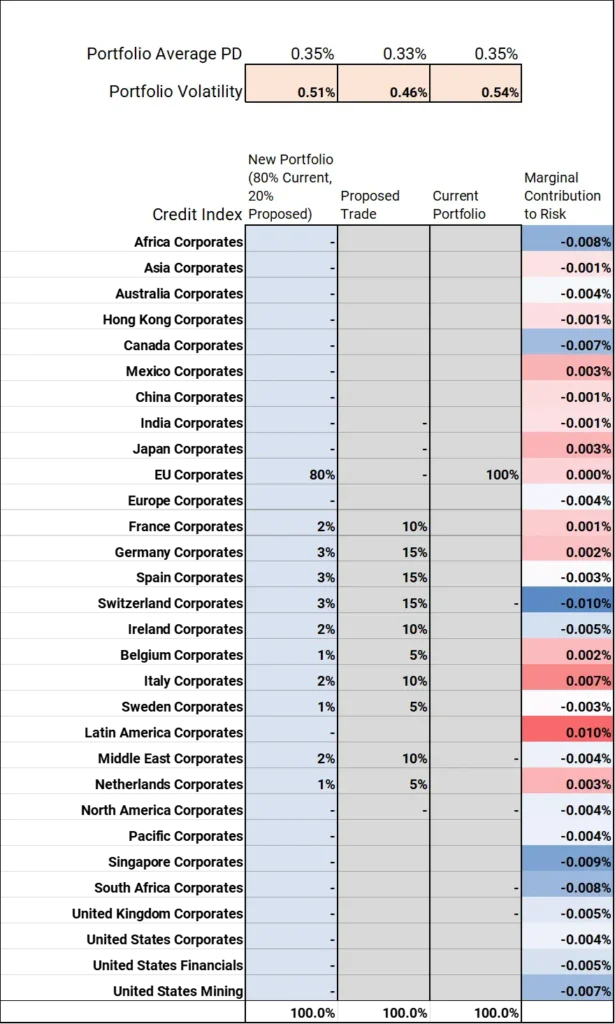
The screenshot below shows a hypothetical portfolio spread across North American and Swiss Corporates with a proposed trade into EU, UK and Middle East Corporates that might diversify risk and increase return.
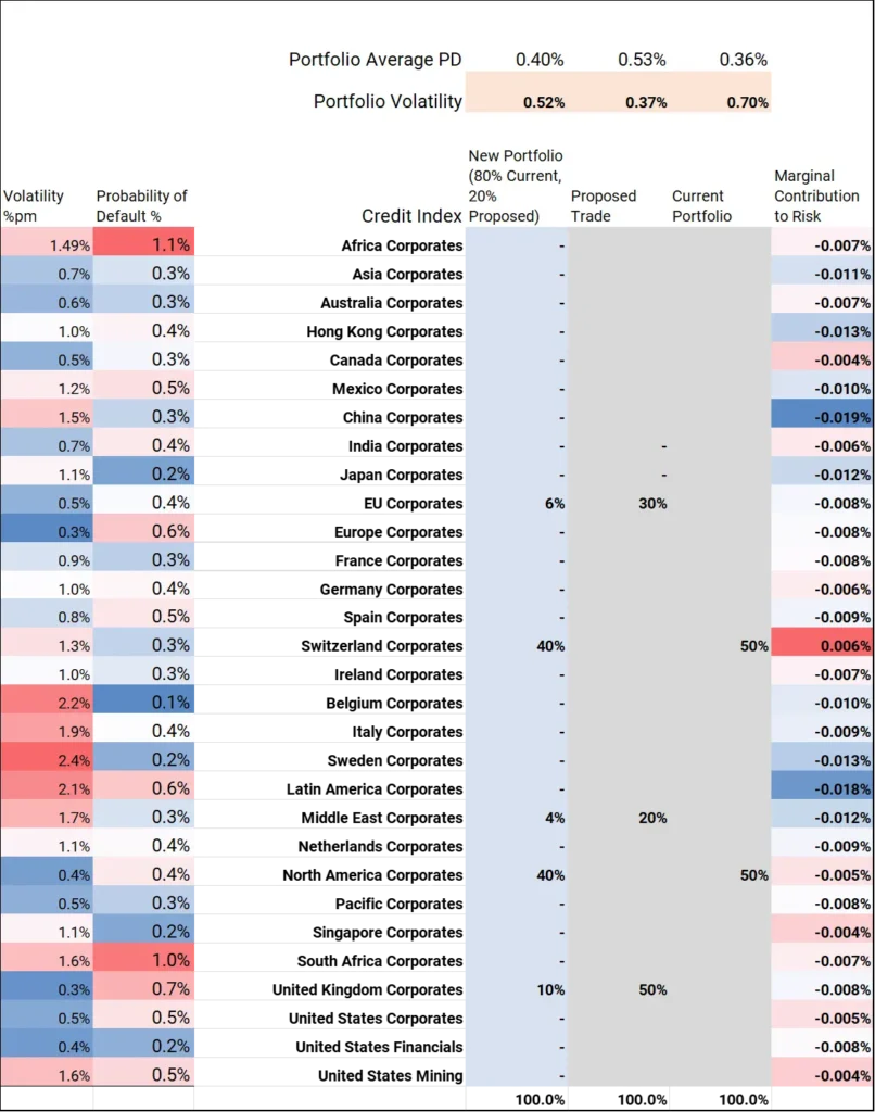
The North America / Switzerland portfolio exposures combined with the credit index correlation and volatilities in the previous exhibit give a monthly PD volatility estimate of 70 basis points and an average portfolio PD of 36 Bps, shown in the rows at the top.
The column on the right is marginal contributions to risk, the effect of a small (+1%) exposure change[3] for the sector credit index in each row.
This shows that there is no scope for adding to Swiss exposure (largest positive marginal contribution); while China and Latin America offer the largest reduction in PD volatility.
The proposed trade has lower PD volatility but a higher PD level (37 and 53 Bps) while the combined portfolio – 80% of the original plus 20% of the new) gives a volatility of 52 Bps and PD of 40 Bps.
Marginal contribution metrics drive portfolio optimization, setting allocations across sectors and assessing the sensitivity of the overall risk number to changes in volatility assumptions, or to correlation matrices based on different historical periods.
5. Portfolio Optimization
The 80/20 mix in the previous example is arbitrary, but the scatterplot below shows the relationship between PD level and PD volatility for various blends of the original portfolio and the proposed trade, using correlations and volatilities from two different periods.
These illustrate the trade-off between default risk and migration risk. A manager may tolerate higher default risk if the migration risk (PD volatility) is low. And it is worth emphasizing that higher consensus PDs may be attractive if loan rate implied PDs are higher. In this case, the chart shows simple mean-variance portfolio optimization.
Past 12 Months
Past 3 Years
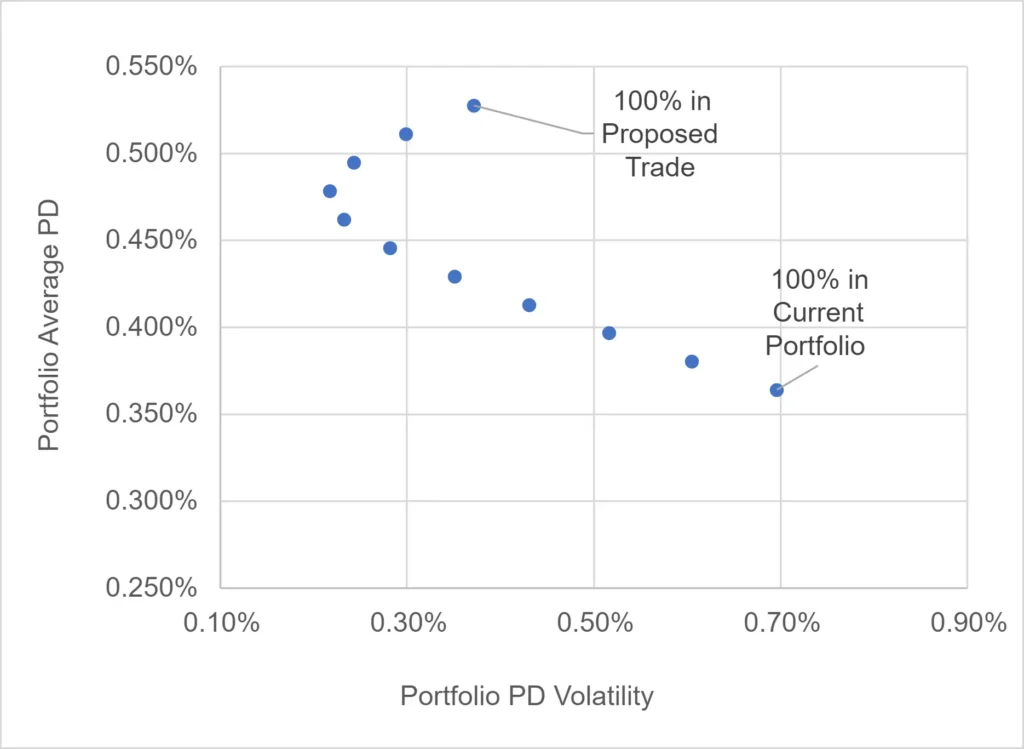
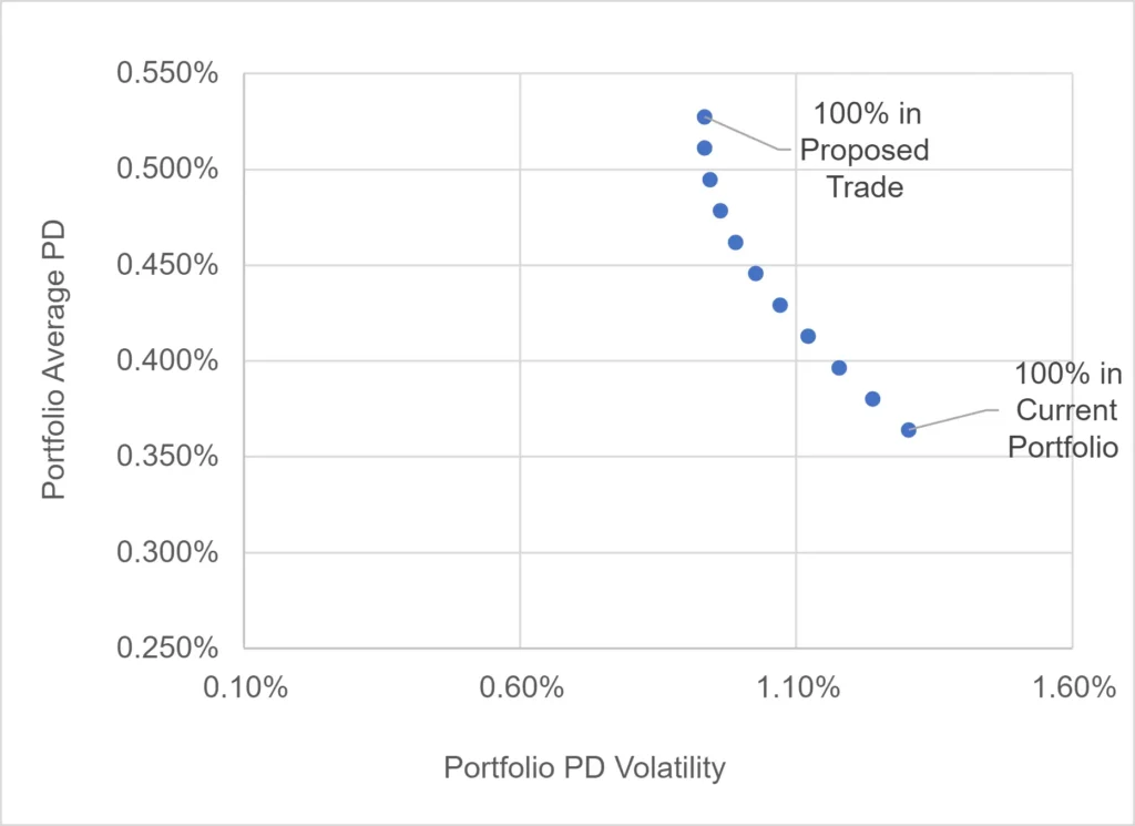
Using PD volatility as the key risk criteria, the recent data plotted on the left suggests a 70% portfolio allocation to the proposed trade (i.e., leaving just 30% in the original portfolio) gives the lowest PD volatility of 22 Bps. But it also represents a major increase in PD level – from 37 Bps to 48 Bps. The three-year data on the right favors a 90% portfolio allocation, but the volatility difference vs. 70% is very small. Based on the recent data, PD volatility is now much more sensitive to the portfolio mix.
So, although an investor may have no control over the country or sector mix in a transaction, there may be scope to scale the investment up or down to achieve a more optimal balance of risk and reward in the credit portfolio.
The next example shows a diversification from 100% in EU Corporates into a mix of EU member nations, plus Switzerland and the Middle East, based on the 12-month correlations and volatilities:
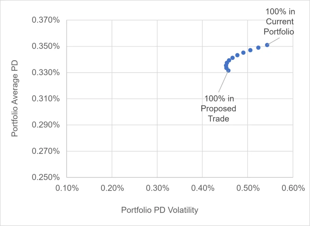
The two portfolios have very similar levels of PD and PD volatility; demonstrating that it is possible to balance the risks of new segments (the Middle East, in this example) with an appropriate mix of exposures to countries that are highly correlated with the original benchmark portfolio (100% EU).
6. Conclusion
Credit Consensus Ratings cover a large universe of borrowers. Credit indices based on these provide more than 1,000 geographic and industry combinations and these provide building blocks for a range of credit risk portfolio metrics. These metrics allow credit portfolio managers to assess risk even without detailed information about individual portfolio constituents; they also support simple portfolio optimization and various sensitivity tests.
To download a worked example Excel template for Credit Index Portfolio Risk, please complete your details:
[1] Ex ante Probability of Default.
[2] Based on monthly % changes in average PDs, for 2020-2022 inclusive.
[3] The balance is taken from the exposures to the other credit indices; these are reduced pro-rata.
[4] Overlapping names in the portfolio and the aggregate, can be handled by the “number of names equivalent” (=n*). n* is calculated as the reciprocal of the sum of squared differences between portfolio holding weights and aggregate constituent weights (A version of the Herfindahl index). Similar calculations can be used for uneven weights.