
October 2017
Credit Index
Download the PDF “Bank-Sourced Credit Indices”
This paper presents a new and unique way of tracking real-world credit risk, using bank-sourced data to construct indices based on forward-looking credit risk estimates.
Indices derived from real-world credit estimates tend to show low correlations with other risk-related macroeconomic data, providing an independent and additive source of data. In addition, unlike market-derived credit risk estimates, real world Probability of Default (“PD”) indices do not contain composite risk premiums * .
Bank-sourced credit data is currently updated monthly. The published obligor-level data set provides One-Year PD estimates for around 12,000 borrowers, based on credit risk estimates from 3 or more banks for each obligor. The indices presented here are based on the much larger mapped dataset, which covers more than 170,000 obligors where at least one bank has contributed a PD.†
Bank-sourced risk estimates provide a frequently updated view of credit trends across a broad set of issuers. This paper discusses some of the challenges presented by bank-sourced credit data and describes the current Credit Benchmark methodology for constructing appropriate indices as well as supporting and derived metrics.
It shows how bank-sourced credit indices can be applied in a number of ways to monitor trends across groups of obligors, as well as in tracking changes in the general level of credit risk. It also shows the correlations between those indices and the volatility of each index, raising the intriguing prospect of monthly credit volatility indices.
There are now a very large number of financial indices available to track the price movements of equities, bonds and derivative metrics across a very large and diverse set of sub-categories. These indices are widely used as benchmarks for portfolio management, and play a pivotal role in the analysis and management of investment performance. With an agreed set of indices, it is possible to decompose portfolio performance into allocation, selection, and timing components.
Some sub-categories consist of similar, near-homogeneous instruments or issuers. For example, a single time series of an index representing UK Short Dated Gilts typically provides a very effective summary of the collective behavior of all UK Government bonds in that maturity category. Other sub-categories are more diverse, and the single index approach can be limiting or even misleading. For example, the movements of oil stocks or overseas earners may at times dominate changes in the S&P500 and FTSE100 indices.
Credit portfolio managers who use investment-style performance and risk measurement frameworks need equivalent metrics for the credit use case. However, the measurement of credit trends across a range of issuers or obligors can be challenging. It is possible to build a foundation of “mirror” credit indices, which track the credit risk of the constituents of standard equity or bond indices. These can be based on stable groups of obligors, and provide a set of base cases for understanding the behaviour of credit indices.
In this paper, we discuss some of the unique characteristics of bank-sourced credit data and illustrate some of the approaches that can be used to track changes across groups of obligors. Index construction rules are proposed along with additional metrics used to assess credit trends in this type of dataset. We present some examples of “mirror” indices, and also introduce some indices based on more dynamic sets of constituents.
N.B. The term “index” is used here primarily in the sense of linked sets of sampled baskets consisting of variable and incomplete groups of equally weighted constituents, with the aim of tracking trends in an underlying universe of legal entities. However, some of the indices discussed in this paper use the more conventional structure of a fixed set of constituents but these are again equally weighted and are only intended to approximate the behaviour of the underlying universe.
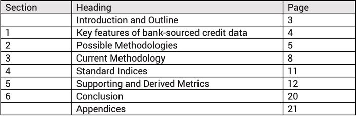
Section 1 looks at the characteristics of bank-sourced credit data and highlights the dynamics and challenges inherent to this type of data. Section 2 discusses various methodological issues in calculating representative index levels. Section 3 presents the proposed CB methodology for index calculation and chain linking indices through time. Section 4 provides a worked example of this methodology and presents the first of what is expected to be a growing set of regularly updated, standardized indices. Section 5 describes supporting metrics that provide additional insight into the behaviour of the constituents of an index. It also discusses derived metrics that can be used to corroborate and calibrate other models. Section 6 summarizes some conclusions from this paper and identifies likely next steps for further research leading to more specialized and bespoke of indices.
Bank lending is a dynamic process, with frequent adjustments to ensure that the structure of credit portfolios reflects the risk and reward objectives of each bank. This can result in trend shifts in the list of specific obligors which feature in typical bank portfolios. Credit indices need to be designed to track these changes in order to provide a relevant peer group benchmark.
In addition to changes in the obligor set, the set of banks providing loans to the same obligor group can also change over time. This dynamism raises statistical issues of survivor bias, selection bias, and like-for-like comparisons. Some examples:
Collectively, the contributing banks in the database can experience significant changes in their loan books each month. This may be due to a decision by an obligor to change bankers; in which case it can result in individual obligors dropping out of the dataset, even if they reappear in the loan books of other banks in subsequent months.
Bank decisions can also result in changes, with obligors dropping out because the lending banks make a conscious decision to not renew their facilities. In either case, the set of up-to-date credit risk estimates for a fixed set of obligors will tend to shrink over time, and the diminishing sample will become increasingly volatile.
This is related to survivor bias. As credit conditions evolve, banks change the structure of their loan books across industries and geographies. They are also likely to change the individual obligors in their loan books as overall credit conditions change.
Over time, changes in credit conditions and credit portfolio objectives will alter the supply, demand and pricing for credit in various industries, geographies and individual names. This will cause variations in the number and identity of banks contributing data for each obligor. In some cases, this may change the average estimates of credit risk for a number of obligors, especially if there are significant differences in the credit risk estimates provided by different banks for the same name.
The next section will address methodology in general, including the selection of the constituent universe. It will also discuss specific approaches for handling the three issues outlined above.
This section discusses the selection of constituents and then reviews the specific adjustments required to address the issues outlined in the previous section.
Index constituents share common characteristics. These may be geographic, industrial or they may be based on specific factors or drivers of share price or business performance. For example, an equity “Value” index is based on dividend yields; a high yield bond index is based on credit risk.‡
The set of possible investment indices is almost unlimited but in practice a limited number of groupings are used based on correlations and dominance. For example, equities and bonds tend to show a low correlation; and the investment choice between these asset classes is more important than the individual instruments in each.
Subdivisions within each asset class are also based on related “clusters” of instruments. For example, bonds may be classified according to short, medium and long duration.
A purely empirical approach would identify related clusters based on correlations, common factors or principal components in the PD data. However in many cases, historic PD data may not be available; common obligor behaviour may need to be inferred from fundamental or classification data.
In credit data, the classification between investment grade and non-investment grade is often the most important dimension. Within these two categories, the industry level may dominate in global businesses (e.g. oil and gas) while the geographic level – especially regional breakdowns – will dominate domestic issuers. As the bank-sourced dataset grows, an increasingly number of indices will be available for different credit, geographic, industry and sector sub-groups.
The indices described in this paper use all relevant mapped obligors in the bank-sourced dataset, whether these are derived from one, two or more than three contributing banks. This is in contrast to the quorate rules used for single name obligor PDs, where the requirement is to use data from at least three contributing banks. The broader data set can be used for indices, because the aggregate nature of the outputs preserves contributor anonymity. In addition, the broader dataset provides a more representative set of indices.
Exhibit 2.2.1 illustrates some of the challenges of using bank-sourced credit data to track trends. This example is based on PDs for a group of airlines over an 18-month period. Each column represents one month; each row represents an airline obligor. If a PD estimate is available for the obligor for a specific month, then the cell at the intersection of the row and column has a value of 1 and the cell is coloured blue; otherwise it is coloured green.
Exhibit 2.2.1 Typical bank-sourced credit data (Airlines sector)
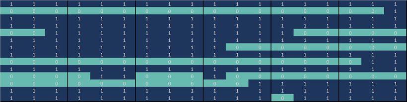
This shows that 7 of these obligors have a continuous series of PDs. All of the others have missing data points. Some of these are isolated instances; others are for extended periods or show intermittent gaps. Exhibit 2.2.1 highlights the issues of survivor bias, selection bias, and lack of like-for-like comparisons. The challenge in building an index from data with these characteristics is to ensure that the essential trends are captured and that optimal use is made of all of the information contained within this heterogeneous dataset.
A pragmatic approach applies an eligibility filter, removing data points that have insufficient history (at least 2 months are required). The remaining data points can be grouped into “baskets” these are sets of constituents which are reset at regular time intervals, maintaining most but not all of the same constituents. The examples in this paper use quarterly basket resets. (See section 3.3. for details)
A credit index level provides a single value summary to track the direction and scale of changes in the credit risk of the constituents. It will typically take the form of an average and there are multiple averaging methods available§ . The most suitable methods are:
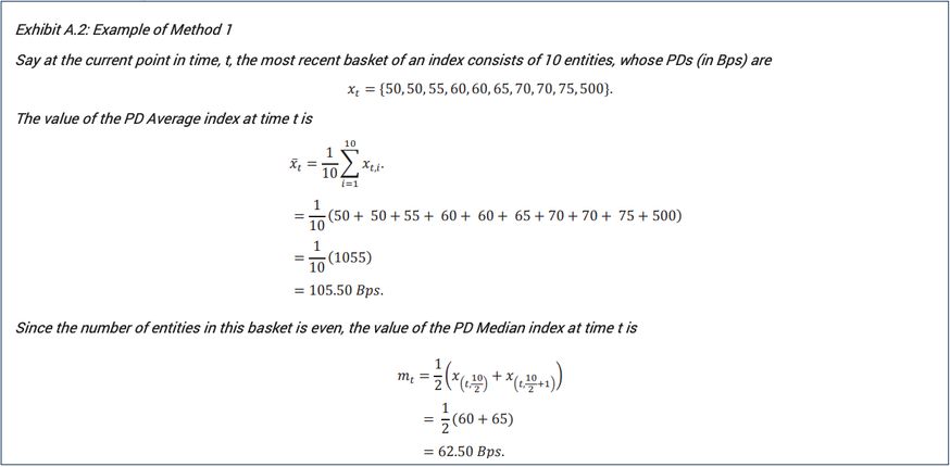
Method 1 – Arithmetic Mean or Simple Median of obligor PD averages. Taking the average of the Probability of Defaults (“PD”) of obligors gives a single index PD with equal weight assigned to each obligor. Taking the median will assign full weight to the obligor PD in the centre of the distribution.
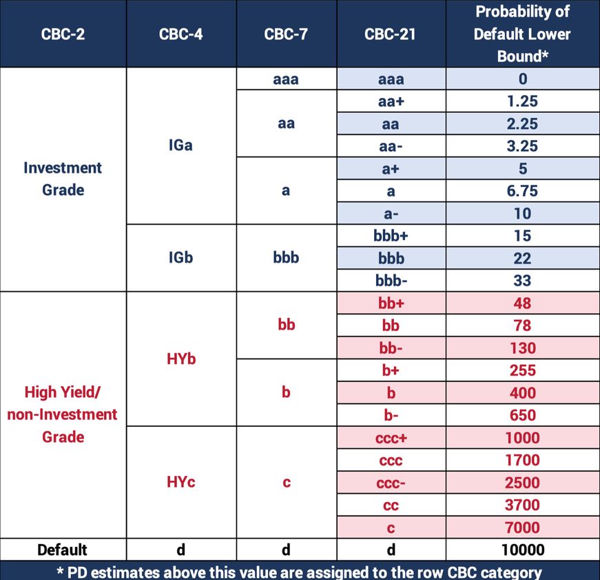
Method 2 – PD equivalent of average of obligor notches, where notches are derived from the obligor PD average using the CBC Scale**Assigning each obligor to a “notch”, approximately based on a log-normal scale††, will reduce the influence of larger PDs.
Exhibit 2.4.1 compares the described methods directly for an EU Retail Index.
Generally, using the arithmetic mean of the PD averages (Method 1) produces an index that has a lower credit quality than that created using the PD averages converted into notches (Method 2). This is expected due to the greater pull a larger PD has on the average in comparison to using its respective notch.
Exhibit 2.4.1: Methods 1 and 2 (EU Retail example)
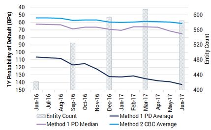
Credit Benchmark currently uses Method 1, as described in the previous section. Both metrics are calculated for each basket, since each has some value in tracking the behaviour of the index constituents. However, for index comparisons in later sections this paper will focus on the Median.
To preserve contributor anonymity and ensure that indices are representative, a number of quorate rules are used.
| Quorate Rules: | |
| A minimum of 4 Banks contributing risk estimates towards the underlying index constituents No contributing bank should be represented in an index by more than 40% of the total contributed observations ‡‡ The minimum number of constituent obligors in an index is 50. |
This is the unweighted sum of each obligor PD (averaged across bank contributions) divided by the number of obligors. For full details see Appendix 2. An alternative approach could be based on the actual contributions; but because multiple banks may provide different estimates for the same obligor, the result would effectively assign more weight to obligors with multiple contributions. The “average of averages” approach assigns equal weight to each obligor, and reduces sampling variation.
This is the central measure of the ordered obligor PD (again after averaging across bank contributions). This is normally at or close to the 50th percentile, depending on whether the number of observations is even or odd. For full details see Appendix 2.
For fixed constituents (the “mirror” indices which reflect an established index such as the Dow Jones 30) the time series construction is straightforward; in effect there is only one overall basket although this will shrink over time as obligors drop out§§ . The median and average of each basket is reported for each monthly publish date.
The basket approach is used to address noise arising from survivor and selection bias, where obligors drop in or out of eligibility across time. Each basket consists of the obligors that are eligible for the index at the time of construction.
| Eligibility Rules: | |
| 1. For Fixed Constituent Indices, all active risk estimates are included in the calculation, including obligors with a single bank contribution. 2. For all CB Indices using basket approaches, the “On the Run” credits are defined as those which at the time of the index rollover have: – A minimum of two contributing banks providing a risk estimate for each obligor. – Three months of consecutive history from the same contributor (with a minimum of 2 contributors) in the quarter coming up to the index rollover month. |
Once constructed, new obligors cannot enter a basket.
Exhibit 3.3.1 illustrates the formation of multiple baskets over time.
Exhibit 3.3.1: Index Benchmark Construction Using Basket-based Series
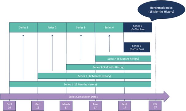
New obligors can enter a new basket, and all currently eligible obligors from the previous basket can also be used in the succeeding basket. While a new basket is formed on a quarterly basis, the index is updated monthly, and hence each basket will be the most current basket for three months.
This period is known as the “On the Run” period of the basket and the index is formed by the “On the Run” values of each basket. Each basket forms its own series, which is also calculated on a monthly basis since its time of construction. The use of multiple baskets addresses the Selection bias issue, by showing the credit quality trends of each specific basket over time.
If a PD contribution drops out, the last valid contribution is rolled over for a maximum of five months, thus the obligor count for each basket is constant for at least its “On the Run” period.
The example in Exhibit 3.3.1 assumes a time series of 15 months, represented by 5 baskets that include the 5th and most recent “On the Run” basket.
Combining these multiple basket outputs into a single adjusted index involves a “Chain Linking” process, which rebases the previous index to the start of a new series (coinciding with the formation of a new basket)*** . This assumes that the change in the new basket would also be observed in the old basket, despite selection effects. (See Appendix 2 for the formalization.)
The published index could be based on initial PD value, final PD value, or somewhere in between. The Credit Benchmark approach currently uses the final PD value as the base. The choice is not critical if the focus is on index changes; if the focus is the index level then the final PD value assumes that the current obligor set is the most representative of current credit risk.
The initial basket series and the final rebased and chain-linked indices form a “sleeve’ representing the boundaries of the index value. It shows the scale of the selection effect; this can vary across different constituent universes (it is worth noting that the Oil & Gas sleeve is wider than most other industries). A set of midpoints can be plotted for each sleeve.
Exhibit 3.4.1: Time Series values for US Oil & Gas Baskets
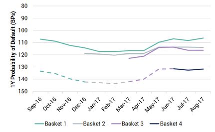
Exhibit 3.4.1 shows four baskets over a 12 month period with an inverted PD scale. The first basket shows a slight deterioration to 117 Bps, before steadily improving beyond 110 Bps and then stabilizing in Q3 2017. The other baskets reflect these moves but each is based at an increasingly lower level of credit quality. The final basket has a value of about 132 Bps and stays relatively stable. In effect, the contributing banks have been steadily extending credit to a more risky set of obligors as credit conditions have improved overall.
Exhibit 3.4.2: US Oil & Gas Index “Sleeve” / Bands and Midpoints (Medians)
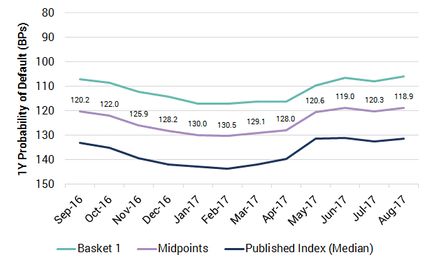
Exhibit 3.4.2 shows the corresponding sleeve (or bands) and midpoints. The midpoints are the best representation of the level of credit quality net of selection effects; the published index shows the current level of credit quality including selection effects. The original basket shows a fixed constituent index (with some survivor bias), with the constituents fixed at the beginning of the display period but dropping out if they do not meet the eligibility criteria.
Exhibit 4.1 shows some of the key standard indices currently produced each month by Credit Benchmark. These represent a mixture of fixed constituent and dynamic, chain-linked indices. These are described as “Credit Quality” metrics (i.e. the inverse of the PD itself). This means that a positive value represents an increase in credit quality or, equivalently, a decline in credit risk / PD.
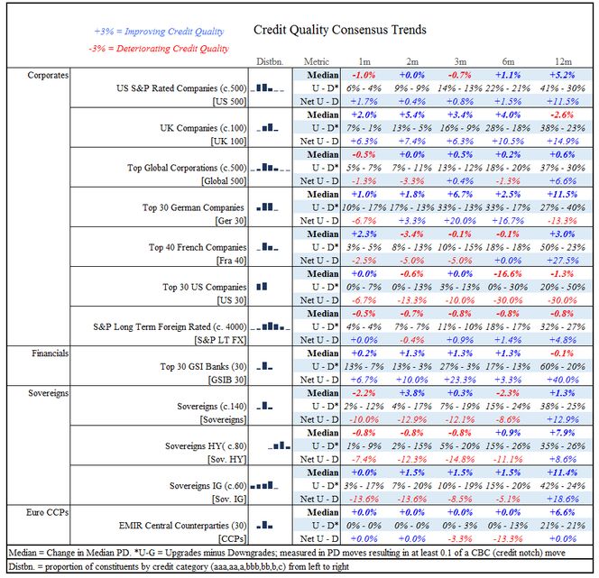
As discussed previously, the basket constituents will fluctuate quarterly; but in general these indices are highly representative of the underlying universe. (Short names in square brackets are used in tables and charts throughout the remained of this paper.)
The main displayed metric is the negative of the change in the median PD of the constituents, where necessary using the chain-linking approach discussed in the previous section. The number in brackets after the index name shows whether the index has fixed constituents (e.g. “(30)”) or dynamic baskets (e.g. (“c.60”)). Some of the additional metrics discussed in the next section are also displayed.
The third column shows the typical distribution of the constituents across the CBC-7 ††† categories. The aaa categories are on the left and the c categories are on the right. For example, EMIR Central Counterparties are typically high quality with the majority in the aa category, and the Top 30 US companies are of higher quality than the Top 40 French companies.
This table shows that, over the past 12 months, median credit risk has improved (the PD has dropped) for most of these obligor groups. This is especially marked for investment grade sovereigns and the top German companies. There has been a slight deterioration in credit quality for the top UK companies but this has reversed in recent months. The top 30 US companies have also declined, especially in the past 6 months and Downgrades have significantly outnumbered Upgrades over the past 12 months, with a similar pattern over more recent periods.
The current methodology reports on median and average changes. The median effectively shows the behaviour of the 50th percentile, (the middle rank of the distribution of obligor credit risks, representing the “typical” obligor). The average measures the “centre of gravity” of the distribution, which can be dominated by a few large observations. These basic measures of group credit risk can be augmented by metrics that provide information about the behaviour of the individual constituents.
For each basket, Upgrades and Downgrades are given by the number of obligors where the PD has changed up or down by more than 0.1 of a CBC notch (See Appendix 1). This shows the balance of the index changes. For example, if there are more upgrades than downgrades while, at the same time, the average index value has decreased, then the index move is dominated by a few obligors. The balance is given by the net figure. There may be months when there are equivalent and large numbers of upgrades and downgrades. For an index to be valuable, it needs to satisfy certain criteria. In particular, credit portfolio managers need to understand the extent to which a given index can be used as a proxy or benchmark for their portfolio. The conventional approach adopted by investment managers uses tracking errors‡‡‡ and this is discussed in detail in Appendix 3.
These show the depth of each basket. If there are large changes in the number of constituents over time then the reported index value needs to be interpreted as having a margin for error. This will be a combination of Credit Distribution differences and Obligor Specific differences. The latter can be measured by the cross sectional volatility of a given basket, discussed in section 5.1.4.
This is the number and proportion of obligors in each broad (CBC-7) credit category across the index constituents. Changes in the index value will primarily be driven by changes in specific credit categories. Credit portfolio managers can compare the credit distribution of their portfolio against that of the benchmark index.
The cross-sectional volatility of a basket is given by the standard deviation of the PD measures for each date. In contrast to equity indices, the cross-sectional volatility of credit estimates can be very high as a proportion of the underlying index. This suggests that the number of obligors in each basket needs to be large if that basket is to be broadly representative of the relevant index.
Effective credit benchmarks should provide a clear indication of changes in trend. The following exhibits show time series of the median PD for the main Corporate and Financial indices discussed in the previous section, and also shows the historic volatility of these time series.
Exhibit 5.2.1.1 Major Corporate and Financial Indices (Medians)
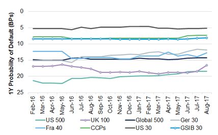
Exhibit 5.2.1.2 Index Relative Volatility, PD Level and Volatility
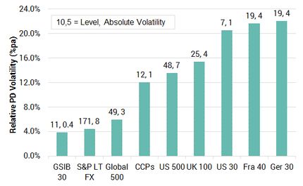
Exhibit 5.2.1.1 shows that the index levels are stable and generally distinct. For example, the typical level of the US 500 index is around 20 Bps whereas the US 30 is around 5Bps. On the other hand, the US 500 also shows evidence of a consistent imrpovement, while the UK 100 deteriorated until Q1 2017 and has started to improve after that point. The other indices have remained within ranges – some wider than others.
Exhibit 5.2.1.2 shows the time series volatility for each of these indices expressed as an average of the index level, and annualised§§§ . The labels show the index level (expressed as a 1Y PD) and the volatility of the index in basis points.
This shows some intuitive as well as some surprising results. For the indices with a limited number of constituents (such as the German 30, the French 40 and the US 30) the proportional volatility is high at around 20%. For the Globally Systemically Important Banks, it is very low – around 4%. The US 500 index shows the highest PD level of 48 Bps, but the standard deviation over the sample period has been moderate at 7 Bps, or about 14%.
This chart is reassuring on the separation issue. The proportionate volatilities are sufficiently low that most indices on this chart will show limited numbers of crossovers unless one or more of them enters a sustained uptrend or downtrend. A high number of crossovers, where two indices repeatedly swap their rankings, is likely to mean that the chosen index basket is too noisy.
Overall, this chart suggests that the historic (time series) volatility of credit risk is not strongly related to the typical level of credit risk. By contrast, the (cross sectional) spread of bank-contributed risk estimates for a given obligor generally shows a strongly positive relationship between level and spread.
For time series volatility measures it is observed that while good credit risks have low PDs, the implication is that any given absolute change in credit risk is proportionately higher. This is similar to some apparently counter-intuitive results observed in the relationship between equity volatility and credit spreads.****
An effective index also needs to distinguish between local and global changes in credit risk. Exhibits 5.2.2.1 to 5.2.2.4 show the relationship between the median index levels of single Country corporates and Global corporates.
Exhibit 5.2.2.1 US vs. Global
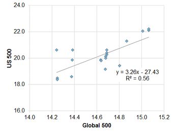
Exhibit 5.2.2.2 France vs. Global
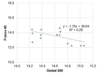
Exhibit 5.2.2.3 UK vs. Global
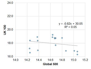
Exhibit 5.2.2.4 Germany vs. Global
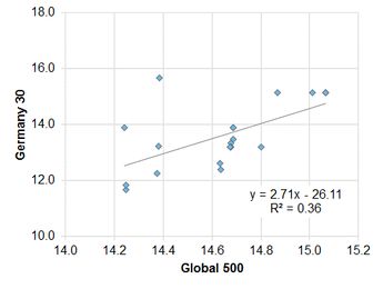
This shows that the strength of the relationship is highly variable. Over the past 18 months, based on median levels, the index of the top 500 US companies shows a moderately positive correlation with the Global 500. This is to be expected given that there will be a large number of companies that are common to both indices.
A smaller sample of German companies is also positively correlated, but the fit is only 36%. French companies show a negative correlation with a fit of 29%; the UK shows no correlation. Running these regressions for changes shows similar results US, UK and France; but the German correlation drops to insignificance. The relationships for averages are weaker, mainly because averages assign more weight to outliers.
This shows that over this period individual indices show considerable divergence. This in turn indicates that the local effect dominated for this set of indices over this period, so the global effect was not strong. This weak common trend component suggests that for this period it is useful to look at correlations between levels as well as the more conventional change-based approach.
The adjusted underlying index levels can be used to estimate correlations and credit index volatilities. Exhibit 5.2.3.1 shows, for the same time period, the correlations and volatilities for levels of the median based indices.
Exhibit 5.2.3.1 Monthly Correlations and Volatilities based on Median Index Levels
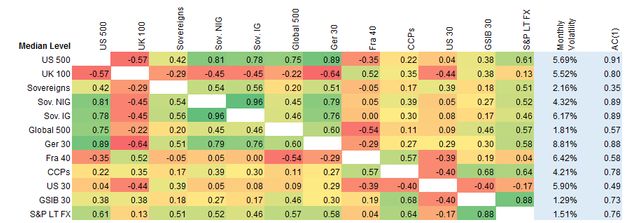
Exhibit 5.2.3.1 shows that, for median levels (correlations are positive unless stated otherwise):
Exhibit 5.2.3.2 shows, for the same time period, correlations and volatilities for changes in the median based indices.
Exhibit 5.2.3.2 Monthly Correlations and Volatilities based on Median Index Changes
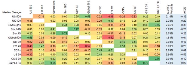
Exhibit 5.2.3.2 shows that, for median changes (correlations are positive unless stated otherwise):
This analysis is based on a limited number of monthly observations so at this stage any conclusions are tentative, but this data suggests:
Correlation and volatility analysis can be extended to adjacent datasets; for example, it is possible to compare credit data with equity indices, bond indices, market volatility measures and macro-economic data. In particular, the Merton model†††† is specified according to equity volatilities; the availability of real world PD estimates provides scope for an alternative set of inputs to that model. This will be explored in future papers.
The Merton model uses equity volatility as an input to estimate the prevailing distance to default. Credit spread volatility is another possible measure‡‡‡‡ . The standard measure of equity volatility is the VIX index§§§§ which is derived from index option prices.
The volatility measures discussed in this paper are based on the entire time series. For comparison with the VIX, rolling PD index volatility has been used as a proxy. This paper uses a 6-month rolling volatility measure to avoid excessive noise.
Exhibit 5.2.5.1 shows the rolling 6 month volatility for the Corporate, Financial and main Sovereign indices.
Exhibit 5.2.5.1 Rolling 6-month volatility, main indices
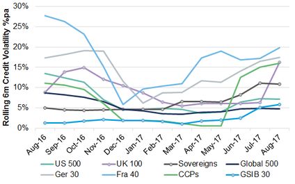
This shows that, over this 13-month period, most of these indices showed a drop in volatility with the low point around the end of 2016. Most of them have shown an increase since then, with France and the UK showing the most dramatic drops and increases. This is a small sample and the 6-month trailing window is short, but it shows that there are clear patterns and trends in credit volatility data based on bank-sourced estimates.
For comparison with the VIX, a Credit Volatility Index is constructed as a simple average of the French, German, US and UK volatility indices. Since the VIX is constructed from options on the S&P500 index, it might be expected that the Credit Volatility Index of US obligors would show the strongest relationship; in practice a multi-country Credit Volatility Index shows the best fit for this short time period.
Exhibit 5.2.5.2 plots the VIX and the Credit Volatility Index as a scatterplot
Exhibit 5.2.5.2 VIX and Credit Volatility Index
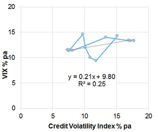
This shows that there is a weak but positive relationship between the Credit Volatility Index and the VIX. The R-squared of 25% implies a correlation of 0.5; statistically significant, but not particularly strong. The points are connected in date order and show a pattern of common movement in time as well as a number of periods when neither metric shows any significant movement. The fitted line shows that the VIX has a positive intercept of 9.8% but the sensitivity to the Credit Volatility Index is only 0.21.
Equity and credit spread volatility effectively measure the volatility of credit risk and the market risk premium; the Credit Volatility Index is a pure measure of the volatility of the real world PD. This may explain why the VIX has a higher baseline volatility (to reflect the volatility of the risk premium itself). Once this effect is removed, the relative insensitivity of the VIX compared with the Credit Volatility Index suggests that the VIX is not fully reflecting changes in the real world PD.
This paper has discussed the advantages and disadvantages of various approaches to the construction of indices for tracking credit risk at the obligor / issuer level.
It has described further details of one of these approaches as the proposed Credit Benchmark methodology and has presented an initial set of standardized indices intended for regular publication. It has also presented various supporting metrics (such as upgrades and downgrades and cross sectional volatility) which provide a detailed understanding of the behaviour of individual index constituents.
Finally, it has shown how indices of this type can be used to analyse correlations between credit indices and track the volatility of those indices.
Let ????????,1, ????????,2, … , ????????,???? be the PDs (averaged across bank contributions) of n entities (obligors), which are the constituents of the current basket at time t.
Order the PD averages at time t such that
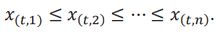
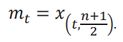
If n is odd, the median will be the ^{th}") PD average:
PD average:
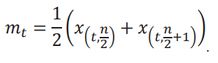
If n is even, the median will be the average of the middle two ordered values:
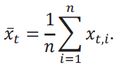
Note that the number of entities, n, can differ from basket to basket. However, while a basket is “On the Run” the value of n is constant. Calculating x̅t and m???? monthly, form the PD Average and PD Median indices, respectively, over time.
This method is not currently used but is often suggested as an alternative to the simple median or average, so the formalized version is shown here for reference. Using the same notation as defined for Method 1, let x????,???? be the PD average of the ith entity, in the most current basket at time t. Using the breakpoints of the CBC-21 Scale (see Appendix 1), this PD can be converted into a “continuous” notch, y????,???? , using linear interpolation. That is,
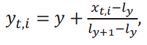
The arithmetic average of y????,1, y????,2, … , y????,????, is calculated, denoted ????̅???? , on a monthly basis. Rearranging Equation [1] to solve for x????,???? , and substituting ????̅???? for ????????,???? the average in notch form reverts back to a PD that is used to form the index.
The chain linking methodology can be formalized as follows:
The chain linking methodology can be formalized as follows:
At time ???? ∈ 3ℕ, where ???? is the time in months from the start of the index, a new basket is to be formed. Define the function ⌊????⌋ as the floor function, which outputs the greatest integer, less than or equal to ????. This basket will be the start of series, which will be “On the Run” during the time periods, t, t + 1, and t + 2. The value of the adjusted indices (AI), calculated between time t and t + 2, at the uth point in time, ???? ∈ [1, t + 2], is calculated by
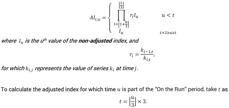
This can be approximated by the formula:
????2???????????????????????????????? ???????????????????? = ????2???????????????????????? + ????2???????????????????????????? + Σ???????????????????? ????????????????????????????s
where:
σCredit = Standard Deviation of Portfolio vs Benchmark attributed to Credit Category mismatches
σObligor = Standard Deviation of Portfolio vs Benchmark attributed to Obligor mismatches
ΣCross Products = sum of interaction terms; if Credit and Obligor risks are independent, then this term is zero
These components are defined as:
σCredit =
where:
where:
is the obligor-specific tracking error in each credit category. This can be estimated from cross sectional volatility, with this element of tracking error approximately inversely proportional to the square root of the number of obligors in the portfolio. | Example of obligor-specific tracking error calculation: | |
| If the annual cross sectional volatility for credit category aa is 100%, and the portfolio has 100 independent obligor exposures, then the Obligor level monthly tracking error for credit category aa is approximately 100% / √100 ≈ 10%. So if the benchmark credit category index PD is 20 Bps, then the portfolio PD will typically lie in the range of 20 +/- 10% ≈ 18-22 Bps. (Although the range is unlikely to be as symmetric in practice due to the typically skewed distribution of PDs.) This is repeated for each credit category and the tracking variances are summed under the assumption of independence. |
The total obligor-level tracking variance is then summed with Credit Category tracking variance. The overall portfolio tracking error is given by the square root of this sum. A number of the components in these calculations can be made available as supporting metrics, as described in Section 5.
Download the article “Bank-Sourced Credit Indices” on PDF.
We aggregate the views of thousands of institutional credit analysts to create new, unique consensus data and analytics. Our clients use the unique entity- and aggregate-level data and analytics to understand and manage their risks effectively. The data helps clients focus their attention on where and when it matters most, whether in their risk management, investment process, or regulatory compliance. Learn more.
Sheliza Siddiqui
Vangelis Koustas
Barbora Makova
Jacob Hibbert
David Carruthers
* This data is “Through-the-Cycle / Hybrid” (TTCH). The other main measure is “Point-in-Time” (PIT) which is more correlated with market prices. TTCH is intended to filter out short term noise but is still sensitive to structural changes in credit risk at the sector or obligor level. It is intended to be a Real World probability measure, whereas Point in Time is closer to a market-implied Risk Neutral probability measure.
† These cannot be published on a single name basis, but they can be grouped into a large and diverse set of index baskets.
‡ As the bank-sourced dataset grows, there will be scope to provide a cluster analysis of the contributed PDs; this will show the full scope for creating credit-tracking indices.
§Including but not restricted to Unweighted or Weighted Mean, Median, Mode, Geometric Mean, and Harmonic Mean.
** See Appendix 1.
††The observed distribution of credit risk data can often be approximated by a lognormal probability density. For this reason, it may be more effective to use a log-normal mean in some applications.
‡‡There is no current minimum % contribution but where necessary this is likely to be set at 10%.
§§For “mirror” indices, the basket will be revised if the constituents of the underlying index are revised by the publishing exchange.
***Note that a more flexible framework applies the basket approach to variable time periods, effectively triggering a new basket whenever new data is available which meets the minimum history criteria.
†††See Appendix 1.
‡‡‡Defined as the standard deviation of the differences in levels (or in some cases the changes) in the PDs of the comparable indices.
§§§The monthly volatilities are annualized using the square root of time adjustment i.e. Annual volatility = Square Root(12) * Monthly volatility.
****“Higher Volatility with Lower Credit Spreads: the Puzzle and Its Solution” A. Semenov, Columbia Business School, August 2016.
††††“On the Pricing of Corporate Debt: The Risk Structure of Interest Rates”. Robert C. Merton, The Journal of Finance, Vol. 29, No. 2 May 1974.
‡‡‡‡ “CDS Spreads Explained with Credit Spread Volatility and Jump Risk of Individual Firms”, A. Kita, January 2012 (10.2139/ssrn.2136458)
§§§§ This is based on prices for current and next month call and put options traded on the S&P 500 index, and is published by the Chicago Board Options Exchange. See http://www.cboe.com/products/vix-indexvolatility
Disclaimer: Credit Benchmark does not solicit any action based upon this report, which is not to be construed as an invitation to buy or sell any security or financial instrument. This report is not intended to provide personal investment advice and it does not take into account the investment objectives, financial situation and the particular needs of a particular person who may read this report.