
1. Credit Correlations
With default risks expected to rise in 2023, correlations between those risks are increasingly important for credit portfolio management. Exposures to different sectors – that normally diversify the portfolio – may show a simultaneous increase in risk during difficult economic conditions. And sectors that are expected to move together may start to diverge.
Consensus credit data, updated twice-monthly, can be used to estimate credit correlations between regions, countries, industries, and sectors. Credit indices (“Aggregates”) track the average probability of default (“PD”) across many constituents[1].
Correlations are typically calculated from percentage changes in average PDs; although the basic time unit is monthly, some users prefer longer time units (e.g. quarterly) with a smaller number of independent timesteps. Correlations can also be calculated for sub-periods, such as pre- and post- COVID; and these can give dramatically different results if the credit regime has shifted from “Risk On” to “Risk Off”.
Figure 1.1 shows two typical credit indices.
Figure 1.1 Credit Index Examples: Global Food & Drug Retailers and Global Automobiles & Parts (Rebased)
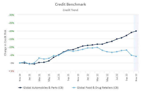
The correlation between these can be calculated by applying the Pearson measure[2] to the monthly percentage changes in average credit risk[3].
Figure 1.1 shows rebased credit indices, starting at a common value in November 2020. The y-axis shows the cumulative percentage change in default risk since then. Correlation calculations are applied to monthly percentage changes in average default probabilities.
Figure 1.2 shows a typical 13 x 13 matrix before and after the COVID pandemic.
Figure 1.2 Credit Correlations, Pre- and Post-COVID
Example: Correlation Matrices between PD changes, pre- and post-COVID
Pre-COVID 2018-2020
Post-COVID 2020-2022
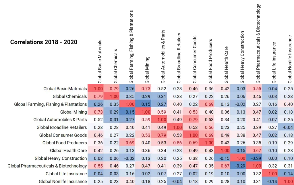
Correlations are much higher after the pandemic, showing that portfolio diversification is particularly difficult to achieve just when it is most needed.
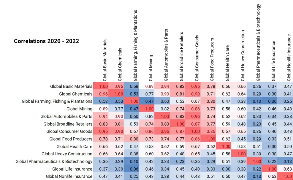
Consensus aggregates cover more than 1,000 country/sector combinations, and most have monthly history back to 2016. Figure 1.3 shows a 30 x 30 matrix for the full period 2016-2022.
Figure 1.3 Credit Correlations, 2016-2022, Various Country/Industry Combinations
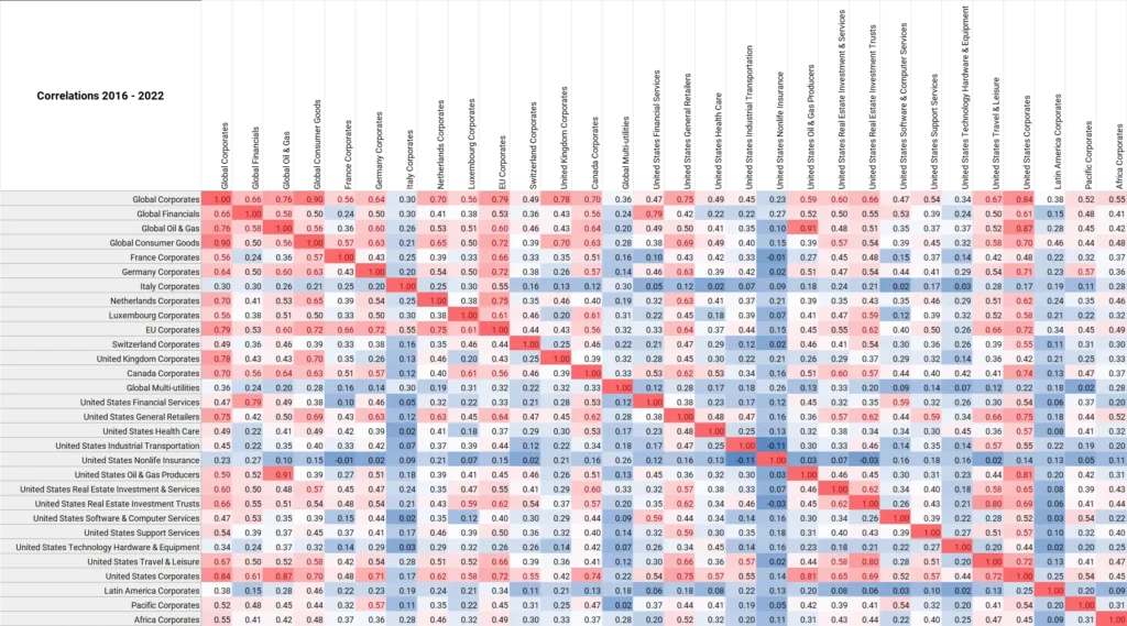
This has been sorted by row/column. Some of the differences in pairwise correlations may be due to the credit distribution within each aggregate: for example, most constituents in one credit index may be mainly investment grade, while others may be heavily skewed towards non-investment grade constituents.
Figure 1.4 shows correlations between broad credit categories (upper and lower investment grade, upper and lower high yield) for Global industries for the period Q4 2018 to Q3 2022.
Figure 1.4 Default Risk Correlations Between Global Industries and Credit Categories, Q4 2018-Q3 2022
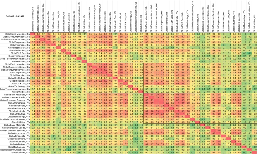
Within each credit category, the average industry correlations are: IGa = 0.50, IGb = 0.59, HYb = 0.69, HYc = 0.31.
This suggests global industry weights may be critical in the highest risk HYc category. This is because credit risk for different industries may show major divergences within that credit group.
By comparison, the upper non-investment grade category HYb shows least scope for diversification by industry. Equally, this means less risk arising from industry concentration; the critical decision here is the portfolio weight assigned to this credit category.
The average correlation between HYb and HYc is 0.32; almost identical to the low correlation across sectors within HYc.
For the period Q2 2021 to Q3 2022, the average correlations in each category are IGa = 0.5, IGb = 0.55, HYb = 0.52, HYc = 0.19. So, scope for diversification has modestly increased in the most recent 18 months, but so has the hazard of sector concentration and single name event risk.

Figure 1.5 plots detailed credit risk correlations between the index of all Global Corporates and the four credit categories for the period Q4 2018 – Q3 2022.
Figure 1.5 Correlation Between Default Probability Changes, All Global Corporates vs. Global Corporate Credit Categories, Monthly, Q4 2018 – Q3 2022
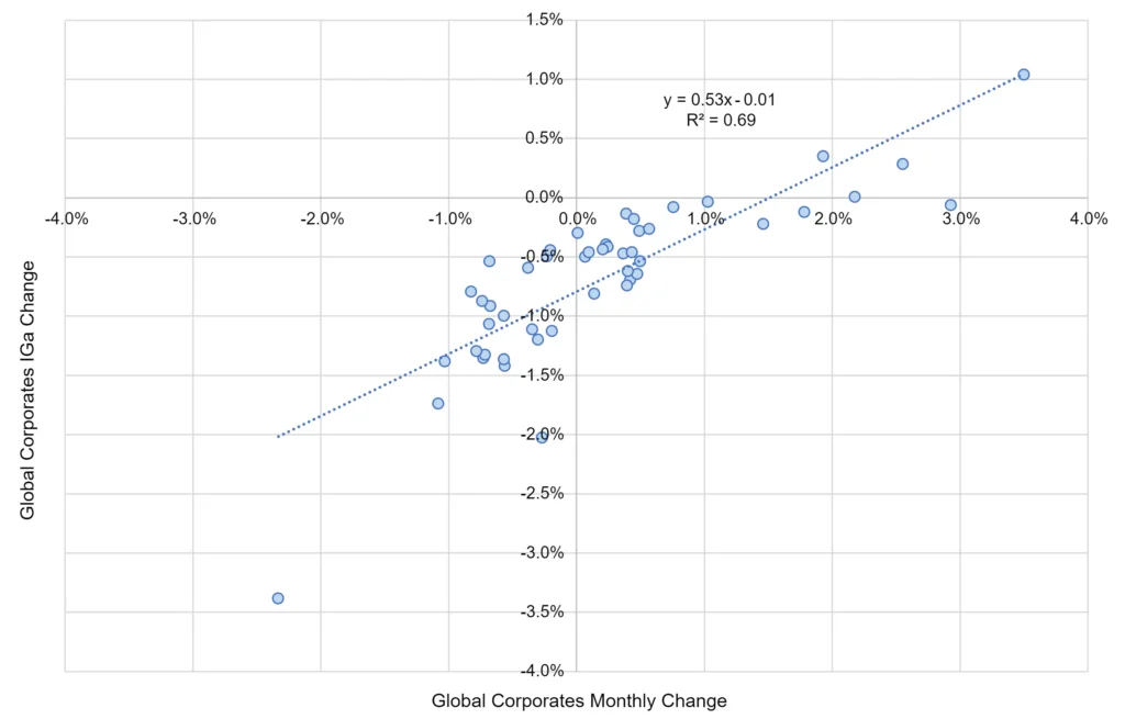
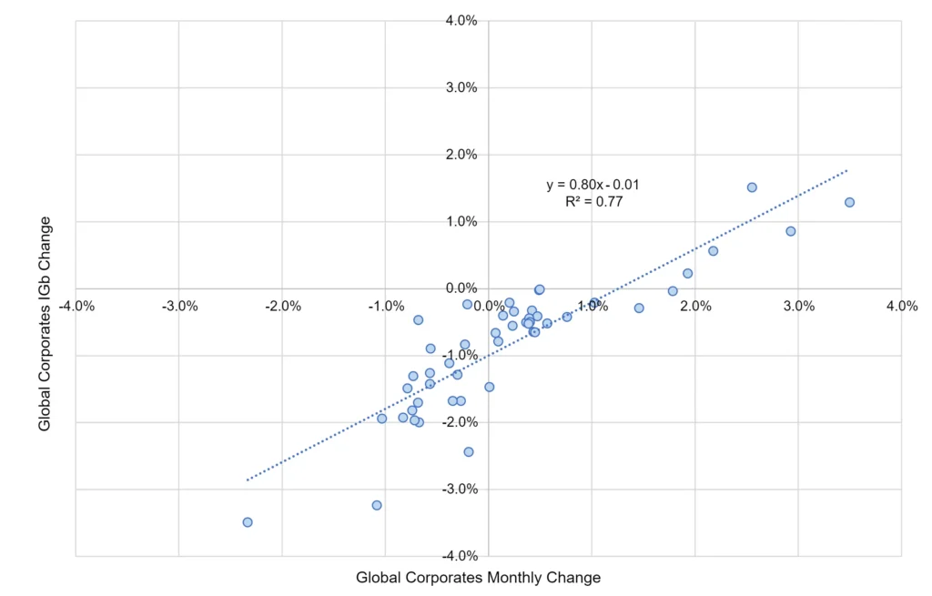
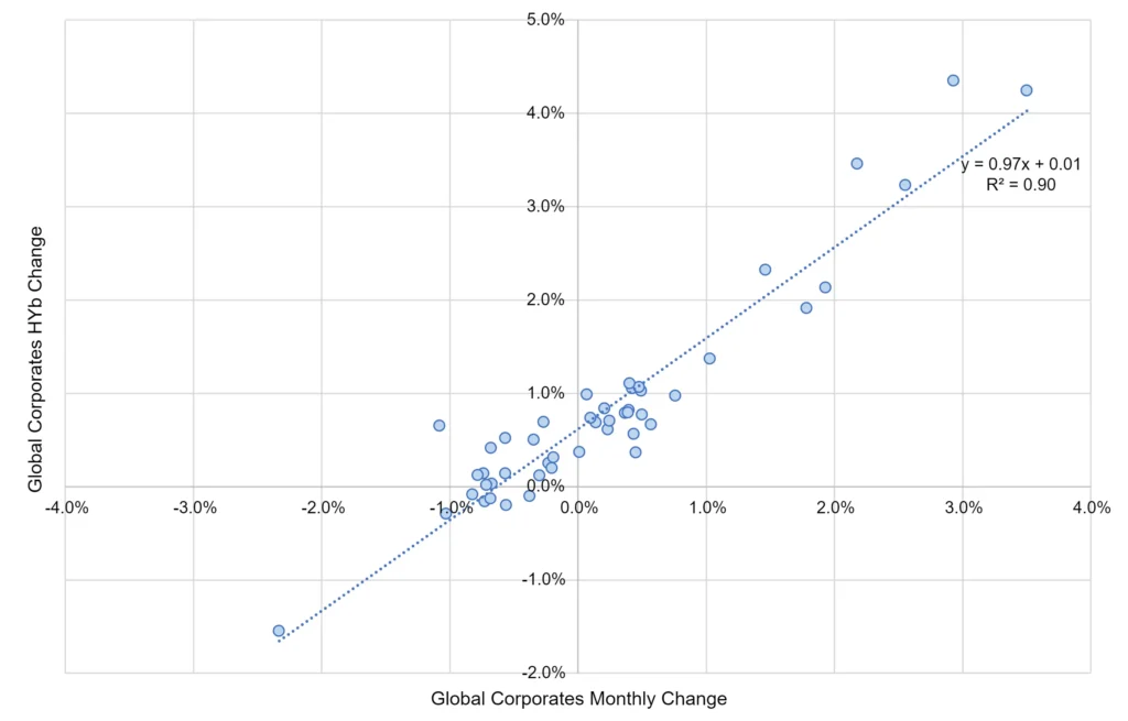
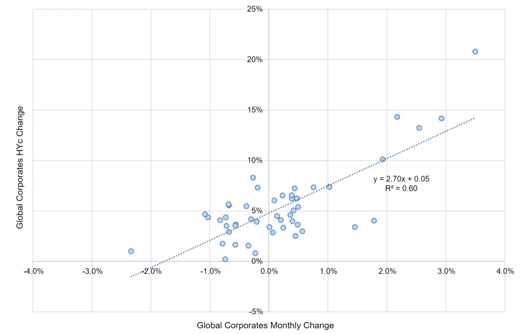
The index of Global Corporate credit risk across all credit categories is very highly correlated with the HYb index (left chart; R2 = 90%), followed by IGb (upper right chart, R2 = 77%). The correlation with IGa is still high (R2 = 69%). The lowest – but still significant – is HYc (R2 = 60%).
These charts can be plotted for all major industries; they alert credit portfolio managers to divergences in credit trends within industries and show the scope for selective diversification from investment grade to high yield. Equally, if the overall credit environment deteriorates, then the lowest quality names will be hardest hit.
While high level geographic and industry/sector credit indices are very useful for tracking broad trends, more detail may be needed for some risk management purposes. In these cases, the correlations between credit category indices shown here may bring added clarity to credit portfolio risk modelling[4].
For managers of structured credit portfolios (such as CLOs), the four credit categories used here approximately correspond to Senior, Upper and Lower Mezzanine, and First Default tranche definitions, so the correlations between them can provide a proxy benchmark for implied correlations quoted in tranche pricing.
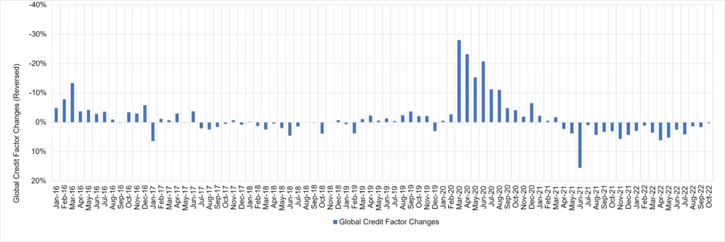
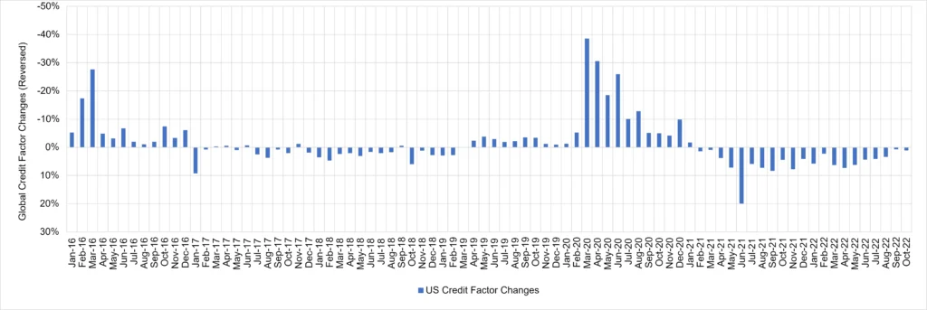
Figure 1.6 shows two versions of the implied time series of changes for largest component. The first is derived from the correlation matrix shown in Figure 1.3; the second is derived from a range of US Industries and Sectors. These are compared with the USD High Yield OAS Level.
Figure 1.6 Common Credit Factor Derived From Different Correlation Matrices vs. HY OAS
Common credit factor derived from mix of Global, US and European Consensus credit indices:
Common credit factor derived from US Consensus credit indices only:
There are differences, but the overall patterns are very similar.
The correlation between changes is 0.96. Option Adjusted Spread, US High Yield:
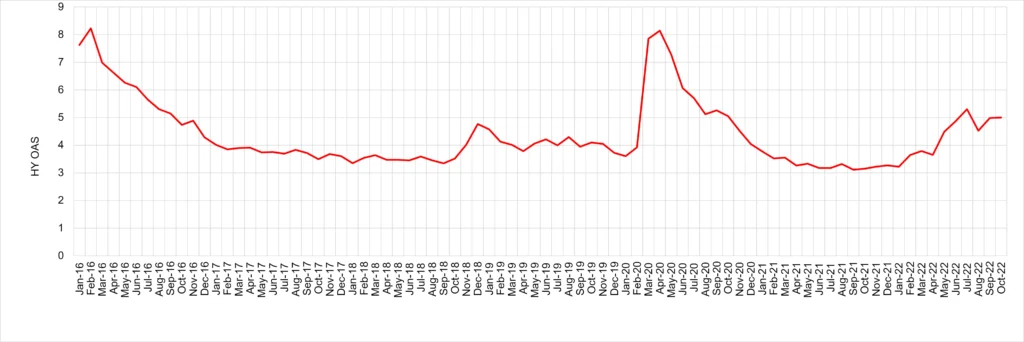
Changes in OAS spreads are not correlated with changes in the common factor or the Global Corporate index. But the major peaks and troughs in the OAS levels are moderately aligned (correlation = 0.6) with common factor changes – suggesting that spikes in market spreads are followed, with a lag, by successive upward revisions in bank risk estimates. If spreads stay high for a sustained period, there will be increasing stress on a growing number of companies.
Different combinations of aggregates result in very similar time series patterns, suggesting a robust “Common Credit Factor”. Reassuringly, changes in this Common Credit Factor are very highly correlated (0.91) with changes in the Global Corporates credit index, so the latter can be used as a proxy for applications like single factor betas, discussed in the next section.
A useful next step is to estimate the sensitivity of country/industry/sector credit indices to the global factor. Figure 1.7 calculates some credit index betas vs. Global Corporates as a proxy for the global factor. Betas are estimated for pre-COVID (2016 – Feb 2020) and post-COVID (July 2020 – Sep 2022).
Figure 1.7 Country / Industry Credit Index Betas vs. Global Corporates, Pre- and Post-COVID
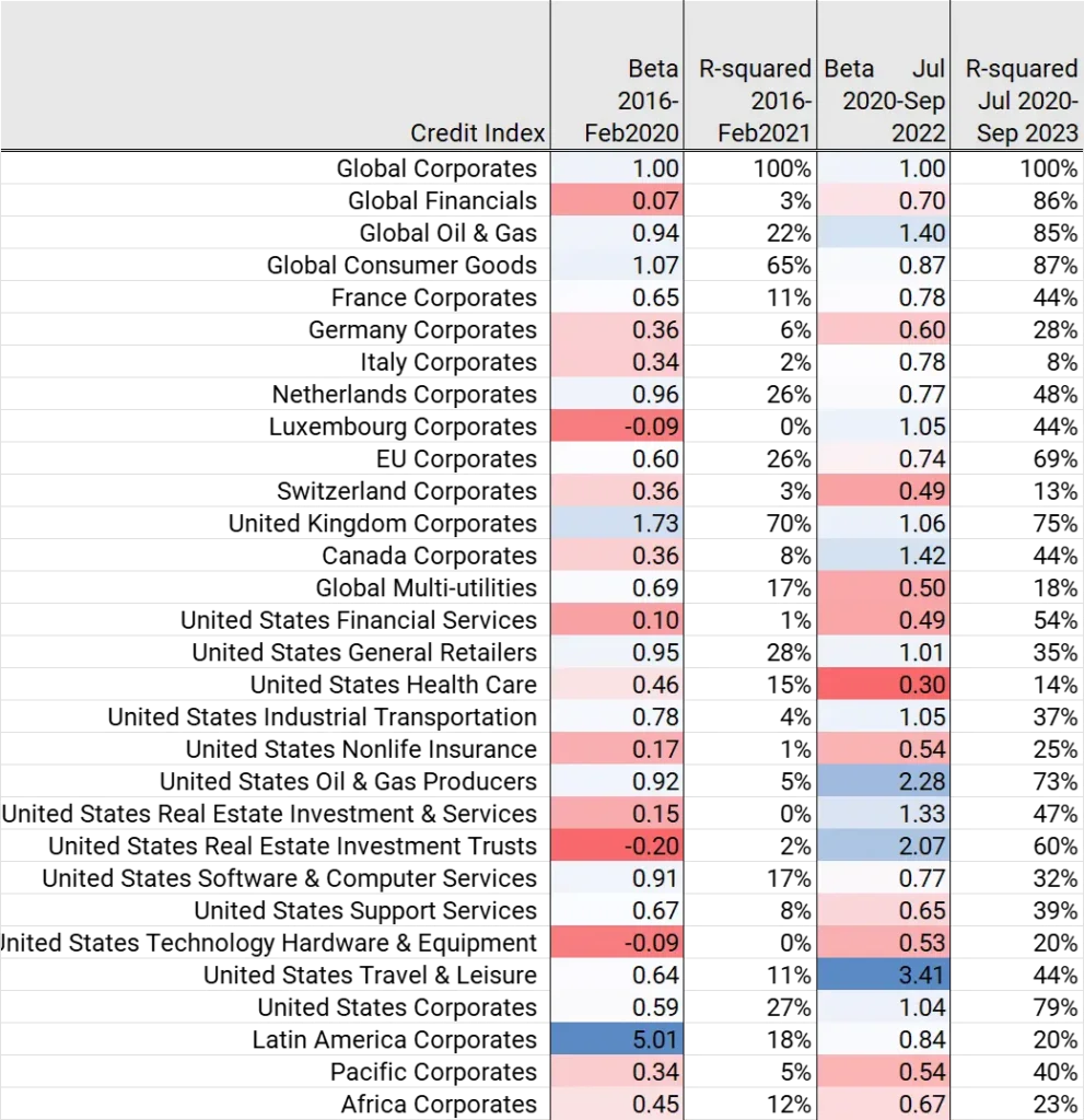
The betas are very different for the two periods. In the pre-COVID period UK Corporates, Latin American Corporates, Global Consumer Goods, US General Retailers, US Oil & Gas and US Software are the highest betas; but most of these have a poor fit (i.e. low correlation with Global Corporates). In the post-COVID period, the higher beta indices include Global Oil & Gas, Canadian Corporates, US Real Estate, and US Travel & Leisure. The average fit is much higher, confirming that industry and country correlations have risen significantly in the post-COVID period, making credit portfolio diversification more challenging.
Betas which show little change over the two periods include Corporates in France and Switzerland, US General Retailers and US Healthcare, US Software and US Support Services, as well as Corporates in Africa and in the Pacific region.
This demonstrates the value of frequent data updates and the need for frequent recalibration of correlations, betas and other risk measures.
2. Use Cases
Credit Portfolio Risk Management:
Any credit risk portfolio can be treated as a set of exposures, with weights adding to at least 100%, and more if leverage is used. PD volatility is one of a large number of metrics that can be used to estimate portfolio credit risk. There are a range of approaches to calibrating this risk, from Monte Carlo simulation (e.g. if exposures are non-linear) to Historic Simulation (very useful when the distribution of asset value changes is not Log-Normal).
Correlation matrices are compact, allowing rapid comparison between many portfolios, and are especially suited to calculating marginal contributions to risk by exposures, as well as portfolio optimization. They can also provide the basis for the Principal Components analysis outlined here. Since they are symmetric, they are most suited to e.g. portfolios with exposures that cluster in the middle of the credit distribution.
For portfolios in the credit tails, it is important to also look at transition matrices, joint default probabilities, and recovery rates.
Financial Stability:
Where two organizations have different exposures to the same underlying set of countries or industries, correlations can be used to assess the joint distribution of their PD volatility – in other words, are the two sets of exposures diversifying or concentrating systemic risks? The same approach can be extended to multiple organizations.
Risk Sharing / Capital Relief Trades:
Investors can use correlation matrices to fine tune deal terms by plotting the risk and reward of alternatives (where offered).
If issuers and investors can agree on a common benchmark correlation matrix (e.g. monthly, calibrated to the past 3 years) they have scope to negotiate pricing with more speed and accuracy to minimize opportunity costs.
Credit category aggregate correlations may be useful for some of these trades, especially if they involve tranches.
For more information, please refer to the whitepaper “Credit Consensus Ratings and Risk Sharing Portfolios”.
Collateralized Loan Obligations (CLOs):
The credit category aggregate correlations reported in this paper can provide a real-world benchmark for implied correlations that feature in CLO tranche pricing.
While correlations between actual issuer risks across credit categories is unlikely to be identical to the correlation between CLO tranches, the matrices shown here should provide a good guide to the expected scale of differences between credit categories.
3. Conclusion
Consensus credit data supports a very large universe of credit risk indices. These cover regions, countries, industries, sectors and credit categories.
Correlations between these can be measured using monthly changes in average default risk estimates. These correlations can be used for credit portfolio risk management purposes, highlighting when a portfolio is at risk from rising credit volatility and – by implication – higher rates of downgrades and defaults.
Further analysis of these correlations reveals a common credit factor, and this is highly correlated with the Global Corporate credit index.
Country and industry regression betas can also be calculated showing the sensitivity of each index to the common factor. Changes in common factor are correlated with Option Adjusted Spread levels, so it is possible to combine bond market spread data with Consensus-based betas to estimate which countries and industries are most at risk from a general increase in credit risk.
So far, the time series data shows two distinct “regimes” separated by the start of the COVID pandemic. Pre-COVID betas are very different from post-COVID betas, illustrating the value of frequent data updates covering large numbers of diverse borrowers.

To access the Appendices of this whitepaper (Principal Components Analysis & Correlation Matrices in Credit Portfolio Risk Calculations), please complete your details to download the full PDF report:
[1] The full history is available as a download from the Reports section of the Credit Benchmark Web Application, and this can be converted (eg via the Excel Pivot functionality) into a large set of time series data for more than 1000 aggregates.
[2] Pearson definition
[3] It can also be applied to the percent change in hazard / survival rates. The results are very similar.
[4] Changes in credit category indices are highly correlated with their parent index: e.g. changes in Global Corporates IGa vs. changes in Global Corporates (All) have a correlation of 0.83. (NB: The chain linking methodology can cause significant drift in the IGa and HYc series, but this does not affect the correlation calculation applied to log differences.)